Creating Report-Ready Charts for Group Comparisons in R: A Step-By-Step Guide
Featuring: The faded violin plot (viofade)
Click here if you just want some code that is ready to copy and paste!
# Load-packages ------------------------------------------------------------------
library(palmerpenguins) # dataset
library(cowplot) # publication-ready plots
library(tidyverse) # ggplot and tidy functions
library(ggdist) # density slabs
library(EnvStats) # stat_n_text() for inserting sample sizes
library(ggtext) # formatting text elements with markdown syntax
library(afex) # anova functions
library(car) # anova functions
library(emmeans) # estimated marginal means and pairwise comparisons
library(effectsize) # effect sizes
library(ggpubr) # significance brackets
library(weights) # rounding values
library(report) # for citing packages
library(janitor) #for cleaning variable names
library(ggpp) # for position_dodge2nudge
# Define color palette
nova_palette <- c("#78AAA9", "#FFDB6E")
# define functions -----------------------------------------------------------
# This function generates a summary table with various statistics for the specified grouping variables and dependent variable.
make_summary <- function(data, dv, grouping1, grouping2, grouping3){
# Use dplyr to group the data by the specified grouping variables and calculate summary statistics
data %>%
group_by({{grouping1}}, {{grouping2}}, {{grouping3}}) %>% # Group by the specified variables
dplyr::summarise(
mean = round(mean({{dv}}), 2), # Calculate and round the mean of the dependent variable
min = round(min({{dv}}), 2), # Calculate and round the minimum
max = round(max({{dv}}), 2), # Calculate and round the maximum
n = n(), # Count the number of observations
std_dev = round(sd({{dv}}), 2), # Calculate and round the standard deviation
se = round(sd({{dv}}) / sqrt(n()), 2), # Calculate and round the standard error
y25 = round(quantile({{dv}}, 0.25)), # Calculate and round the 25th percentile
y50 = round(median({{dv}})), # Calculate and round the median (50th percentile)
y75 = round(quantile({{dv}}, 0.75)), # Calculate and round the 75th percentile
loci = round(mean({{dv}}), 1) - 1.96 * se, # Calculate and round the lower confidence interval
upci = round(mean({{dv}}), 1) + 1.96 * se # Calculate and round the upper confidence interval
)
}
#We can make a custom function calculate_and_merge_effect_sizes() to loop compute cohen’s d for each comparison, then merge the effect sizes in our flipper_emmeans_contrasts dataframe:
calculate_and_merge_effect_sizes <- function(emmeans, model) {
contrasts <- data.frame(emmeans$contrasts)
emmean_d <- data.frame(emmeans::eff_size(
emmeans,
method = "pairwise",
sigma = sigma(model),
edf = df.residual(model)))
combined_dataframe <- data.frame(contrasts, emmean_d)
# Rename some columns for clarity
combined_dataframe <- combined_dataframe %>%
select(-contrast.1, -df.1)%>%
rename(d = effect.size,
d_ci_low = lower.CL,
d_ci_high = upper.CL,
d_se = SE.1,
df_error = df,
p = p.value)
# Return the combined dataframe with effect size results
return(combined_dataframe)
}
# Make a custom function, merge_emmeans_summary(), to merge summary and emmeans. Particularly useful for multivariate analyses:
#merging regular summary stats with emmeans
# This function takes summary data and a tidy emmeans object and adds emmeans-related columns to the summary data
merge_emmeans_summary <- function(summary_data, emmeans_tidy) {
# Add emmeans-related columns to the summary_data
# Assign the 'emmean' values from the emmeans_tidy to a new column 'emmean' in summary_data
summary_data$emmean <- emmeans_tidy$emmean
# Assign the 'SE' values from emmeans_tidy to a new column 'emmean_se' in summary_data
summary_data$emmean_se <- emmeans_tidy$SE
# Assign the 'lower.CL' values from emmeans_tidy to a new column 'emmean_loci' in summary_data
summary_data$emmean_loci <- emmeans_tidy$lower.CL
# Assign the 'upper.CL' values from emmeans_tidy to a new column 'emmean_upci' in summary_data
summary_data$emmean_upci <- emmeans_tidy$upper.CL
# Return the summary_data with the added emmeans-related columns
return(summary_data)
}
# This function generates a text summary based on user-specified options using a tidy t-test dataframe.
report_tidy_t <- function(tidy_frame,
italicize = TRUE,
ci = TRUE,
ci.lab = TRUE,
test.stat = FALSE,
point = TRUE,
pval = TRUE,
pval_comma = TRUE
){
# Initialize an empty string to store the result text
text <- ""
# Conditionally add effect size (d) to the result text
if (point == TRUE) {
text <- paste0(text,
ifelse(italicize == TRUE, "*d* = ", "d = "), # Italicized or not
round(tidy_frame$d, 2) # Rounded d value
)
}
# Conditionally add 95% CI to the result text
if (ci == TRUE) {
text <- paste0(text,
ifelse(ci.lab == TRUE,
paste0(", 95% CI [",
round(tidy_frame$d_ci_low, 2), ", ",
round(tidy_frame$d_ci_high, 2), "]"), # Label and rounded CI values
paste0(" [",
round(tidy_frame$d_ci_low, 2), ", ",
round(tidy_frame$d_ci_high, 2), "]") # Only rounded CI values
)
)
}
# Conditionally add t-statistic and degrees of freedom to the result text
if (test.stat == TRUE) {
text <- paste0(text,
", *t*(", round(tidy_frame$df_error, 2), ") = ", round(tidy_frame$t, 2) # t-statistic and df
)
}
# Conditionally add p-value to the result text
if (pval == TRUE) {
text <- paste0(text,
ifelse(pval_comma == TRUE,
ifelse(italicize == TRUE, ", *p* ", ", p "),
ifelse(italicize == TRUE, "*p* ", "p ") # Italicized or not
),
ifelse(tidy_frame$p < .001, "< .001", # Formatting based on p-value
ifelse(tidy_frame$p > .01,
paste("=", tidy_frame$p %>% round(2)),
paste("=", tidy_frame$p %>% round(3))
)
)
)
}
# Return the generated text summary
return(text)
}
# This function formats a p-value and optionally italicizes it for reporting.
report_pval_full <- function(pval, italicize = TRUE) {
# Check if the p-value is less than .001
if (pval < .001) {
# If p-value is very small, format it as "*p* < .001" (with or without italics)
result <- ifelse(italicize == TRUE, "*p* < .001", "p < .001")
} else {
# If p-value is not very small, format it as "*p* = " with either 2 or 3 decimal places
if (pval >= .01) {
# Use 2 decimal places for p-values >= .01
result <- ifelse(italicize == TRUE, "*p*", "p") # Start with "*p*" or "p"
result <- paste0(result, " = ", weights::rd(pval, 2)) # Append the formatted p-value
} else {
# Use 3 decimal places for p-values less than .01
result <- ifelse(italicize == TRUE, "*p*", "p") # Start with "*p*" or "p"
result <- paste0(result, " = ", weights::rd(pval, 3)) # Append the formatted p-value
}
}
# Return the formatted p-value
return(result)
}
# This function generates a text summary of ANOVA results based on user-specified options.
report_tidy_anova_etaci <- function(tidy_frame, # Your tidy ANOVA dataframe
term, # The predictor in your tidy ANOVA dataframe
effsize = TRUE, # Display the effect size
ci95 = TRUE, # Display the 95% CI
ci.lab = TRUE, # Display the "95% CI" label
teststat = TRUE, # Display the F-score and degrees of freedom
pval = TRUE # Display the p-value
){
# Initialize an empty string to store the result text
text <- ""
# Conditionally add effect size (eta square) to the result text
if (effsize == TRUE) {
text <- paste0(text,
"\u03b7^2^ = ", # Unicode for eta square
round(as.numeric(tidy_frame[term, "pes"]), 2)
)
}
# Conditionally add 95% CI to the result text
if (ci95 == TRUE) {
text <- paste0(text,
ifelse(ci.lab == TRUE,
paste0(", 95% CI ["), " ["),
round(as.numeric(tidy_frame[term, "pes_ci95_lo"]), 2), ", ",
round(as.numeric(tidy_frame[term, "pes_ci95_hi"]), 2), "]"
)
}
# Conditionally add F-score and degrees of freedom to the result text
if (teststat == TRUE) {
text <- paste0(text,
", *F*(", tidy_frame[term, "Df"],
", ", tidy_frame["Residuals", "Df"], ") = ",
round(as.numeric(tidy_frame[term, "F.value"], 2))
)
}
# Conditionally add p-value to the result text
if (pval == TRUE) {
text <- paste0(text,
", ", report_pval_full(tidy_frame[term, "Pr..F."])
)
}
# Return the generated text summary
return(text)
}
# load-data ------------------------------------------------------------------
# assigns data to a dataframe we call "df"
df <- palmerpenguins::penguins
# drop rows with missing values
df <- df[complete.cases(df)==TRUE, ]
df <- rename(df, flipper = flipper_length_mm)
# peek at the structure of our dataframe
str(df)
# create summary dataframe --------------------------------------------
# Apply our custom function to create summary dataframe
flipper_summary <- make_summary(data = df, dv = flipper, grouping1 = species)
# Show summary dataframe in table
knitr::kable(flipper_summary)
# analysis ------------------------------------------------------------------
# Anova with stats::aov() and car::Anova():
# Fit data
flipper_fit <- stats::aov(flipper ~ species, data = df)
# Run anova
flipper_anova <- car::Anova(flipper_fit)
#Calculate effect sizes with effectsize::eta_squared(), and import them into the ANOVA table:
# Extract effect size (partial eta squared) from anova
flipper_anova_pes <- effectsize::eta_squared(flipper_anova,
alternative="two.sided",
verbose = FALSE)
# Convert anova table into dataframe
flipper_anova <- data.frame(flipper_anova)
# import effect size estimates and confidence intervals to anova dataframe
flipper_anova$pes_ci95_lo <- flipper_anova_pes$CI_low
flipper_anova$pes_ci95_hi <- flipper_anova_pes$CI_high
flipper_anova$pes <- flipper_anova_pes$Eta2
# round all numeric columns to 2 decimal places
flipper_anova <- flipper_anova %>%
dplyr::mutate_if(is.numeric, function(x) round(x, 2))
# display anova dataframe
knitr::kable(flipper_anova)
# Estimated marginal means --------------------------
# Extract estimated marginal means
flipper_emmeans <- emmeans::emmeans(flipper_fit, specs = pairwise ~ species)
# convert estimated marginal mean contrasts to dataframe
flipper_emmeans_contrasts <- data.frame(flipper_emmeans$contrasts)
# Convert estimated marginal means to dataframe
flipper_emmeans_tidy <- data.frame(flipper_emmeans$emmeans)
# Use merge_emmeans_summary() to combine with our basic flipper_summary into a single model-enhanced dataframe:
# Order the dataframes based on dependent variables - Not necessary here, but good practice that helps for factorial designs
flipper_summary <- flipper_summary[order(flipper_summary$species), ]
flipper_emmeans_tidy <- flipper_emmeans_tidy[order(flipper_emmeans_tidy$species), ]
# merge dataframes
flipper_summary <- merge_emmeans_summary(summary_data = flipper_summary,
emmeans_tidy = flipper_emmeans_tidy)
# Round numeric values
flipper_summary <- flipper_summary %>%
mutate_if(is.numeric, function(x) round(x, 2))
flipper_summary
#merge estimated marginal mean contrasts with their effect sizes:
flipper_emmeans_contrasts <- calculate_and_merge_effect_sizes(flipper_emmeans, flipper_fit)
flipper_emmeans_contrasts
# visualize data -------------------
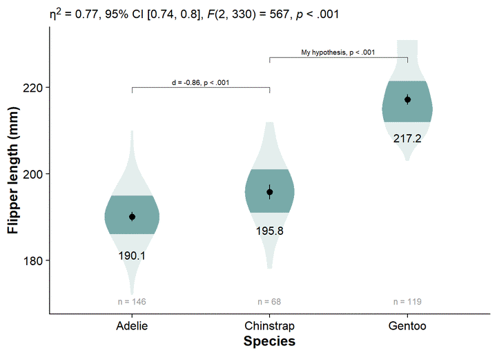
ggplot(data = df, # specify the dataframe that we want to pull variables from
aes(y = flipper, # our dependent/response/outcome variable
x = species # our grouping/independent/predictor variable
)) +
cowplot::theme_half_open() + # nice theme for publication
ggdist::stat_slab(side = "both", # turn from slab to violin
aes(fill_ramp = stat(level)), # specify shading
fill = nova_palette[1], # specify used to fill violin
.width = c(.50, 1), # specify shading quantiles
scale = .4) + # change size of violin
geom_pointrange(data = flipper_summary, # our externally-defined summary dataframe
aes(x = species, # our independent variable
y = mean, # our outcome/dependent variable
ymin = loci, # lower-bound confidence interval
ymax = upci # upper-bound confidence interval
)) +
geom_text(data = flipper_summary, aes(x = species,
y = mean,
label = round(mean,1)),
color="black",
size = 2.5,
vjust = 5) +
geom_text(data = flipper_summary,
aes(label = paste("n =", n),
y = flipper_summary[which.min(flipper_summary$min),]$mean -
3*flipper_summary[which.min(flipper_summary$min),]$std_dev), # dynamically set the location of sample size (3 standard deviations below the mean of the lowest-scoring group)
size = 2,
color = "grey60") +
guides(fill_ramp = "none") + # get rid of legend element for fading quantiles
labs(subtitle = report_tidy_anova_etaci(flipper_anova,"species")) +
theme(plot.subtitle = ggtext::element_markdown()) +
ggpubr::geom_bracket(
tip.length = 0.02, # the downard "tips" of the bracket
vjust = 0, # moves your text label (in this case, the p-value)
xmin = 1, #starting point for the bracket
xmax = 2, # ending point for the bracket
y.position = 220, # vertical location of the bracket
label.size = 2.5, # size of your bracket text
label = paste0(
report_tidy_t(
flipper_emmeans_contrasts[flipper_emmeans_contrasts$contrast =="Adelie - Chinstrap",],
italicize = FALSE,
ci = FALSE)) # content of your bracket text
) +
ggpubr::geom_bracket(
tip.length = 0.02,
vjust = 0,
xmin = 2,
xmax = 3,
y.position = 227 ,
label.size = 2.5,
label = paste0("My hypothesis, ",
report_tidy_t(flipper_emmeans_contrasts[flipper_emmeans_contrasts$contrast =="Chinstrap - Gentoo",],
italicize = FALSE,
ci = FALSE,
point = FALSE,
pval_comma= FALSE))
# label = paste0("My hypothesis, ",
# report_pval_full(flipper_emmeans_contrasts[flipper_emmeans_contrasts$contrast ==
# 'Chinstrap - Gentoo', "p"], italicize = FALSE))
#
)+
theme(axis.title = element_text(face="bold")) +
ylab("Flipper length (mm)") +
xlab("Species")
ggsave(here::here("figures", "viofade.png"),
width=7, height = 3, dpi=700)
I have been enjoying making some guides for data visualization, namely trying to improve on the raincloud plot via the new fadecloud as well as faded dotplots and shadeplots. However, I want to make sure that all users have the chance to easily begin using all of the many great tools in ggplot to create figures that are ready for publication. This post is a rundown of a workflow that I use for preparing group-comparison graphs that are ready to include in nearly any kind of report.
In addition to being a personal resource, this post is intended to be more accessible for newcomers to the R and ggplot ecosystems. Although I assume a working understanding of R, this post is sectioned out piece-by-piece to better demonstrate the impacts of each function and argument for ggplot.
Free Learning Resources
With newcomers in mind, here are some no-cost resources
- R fundamentals
- R for Data Science (2e)
- Prime Hints For Running A Data Project In R
- How to organize your analyses with R Studio Projects
- What They Forgot to Teach You About R
- The tidyverse style guide
- Functions
- Reproducible Analysis With R
- R Workflow blog post and e-book
- Data Skills for Reproducible Research
- Beyond Basic R - Introduction and Best Practices
- Data visualization with ggplot2 :: Cheat Sheet
- How to Structure RStudio Projects
- Organising Data in R
- Stats
- Statistical rethinking with brms, ggplot2, and the tidyverse
- Statistical Rethinking videos
- One Way ANOVA with R
- Understanding Statistical Power and Significance Testing: an interactive visualization
- easystats package
- Statistics: Data analysis and modelling
- Analysis of Factorial Designs foR Psychologists
- Guide to Effect Sizes and Confidence Intervals
- ggstatsplot package
Notes on the Workflow
After a few projects, I have found that I get my best results by summarizing and analyzing my data before trying to create any publication-ready visualizations. There are a few benefits:
- This process automatically creates the graph with the most up-to-date test statistics, all in a reproducible and portable process. Otherwise, when you make changes, you visualize, run the analysis, and have to go back and manually update any revised stats in the plot. Similarly, if your significance tests are done as part of your plotting (e.g., with r package
ggsignif, you can end up struggling with making sure your in-text and graphed statistical tests match.
- You can easily use this process to visualize estimated marginal means, which are a product of your statistical model. This allows you to match your statistics to the visualized data.
- Summary data is often needed for reporting and extra scripting functions. Instead of having to go back to your scripts to get summary statistics, they are readily and consistently available as part of your data processing and analysis.
- This workflow is easily adapted to multivariate and univariate analyses, potentially cutting down on time and decisions down the road.
Please do not take this guide as license to start summarizing and analyzing your data without properly exploring and cleaning it. This workflow is intended for creating the final product (i.e., after you have screened for influential observations, missingness, etc.).
Load Packages
library(palmerpenguins) # dataset
library(cowplot) #  publication-ready plots
library(tidyverse) # ggplot and tidy functions
library(ggdist) # density slabs
library(EnvStats) # stat_n_text() for inserting sample sizes
library(ggtext) # formatting text elements with markdown syntax
library(afex) # anova functions
library(car) # anova functions
library(emmeans) # estimated marginal means and pairwise comparisons
library(effectsize) # effect sizes
library(ggpubr) # significance brackets
library(weights) # rounding values
library(report) # for citing packages
library(janitor) #for cleaning variable names
library(ggpp) # for position_dodge2nudge

# Define color palette
nova_palette <- c("#78AAA9", "#FFDB6E")
Load Data

We’ll use the palmerpenguins::penguins dataset, which is easy to get running right away:
# assigns data to a dataframe we call "df"
df <- palmerpenguins::penguins

# drop rows with missing values
df <- df[complete.cases(df)==TRUE, ]

df <- rename(df,  flipper = flipper_length_mm)

# peek at the structure of our dataframe
str(df)
## tibble [333 x 8] (S3: tbl_df/tbl/data.frame)
##  $ species       : Factor w/ 3 levels "Adelie","Chinstrap",..: 1 1 1 1 1 1 1 1 1 1 ...
##  $ island        : Factor w/ 3 levels "Biscoe","Dream",..: 3 3 3 3 3 3 3 3 3 3 ...
##  $ bill_length_mm: num [1:333] 39.1 39.5 40.3 36.7 39.3 38.9 39.2 41.1 38.6 34.6 ...
##  $ bill_depth_mm : num [1:333] 18.7 17.4 18 19.3 20.6 17.8 19.6 17.6 21.2 21.1 ...
##  $ flipper       : int [1:333] 181 186 195 193 190 181 195 182 191 198 ...
##  $ body_mass_g   : int [1:333] 3750 3800 3250 3450 3650 3625 4675 3200 3800 4400 ...
##  $ sex           : Factor w/ 2 levels "female","male": 2 1 1 1 2 1 2 1 2 2 ...
##  $ year          : int [1:333] 2007 2007 2007 2007 2007 2007 2007 2007 2007 2007 ...
For your own real-life data importing, the function you use depends on your file type. I usually use the following: readr::read_csv() (csv files), readxl::read_excel() (excel files), or haven::read_sav() (SPSS files).
You can find tutorials for data importing at:
One of the tricky parts of data importing is defining the right paths to your data. Best practice is to use RStudio Projects, and use a consistent subfolder scheme for organizing your data/output/figures/reports/etc.
For project organization schemes, see:
Summarize the Data
make_summary is my workhorse custom function for any group comparison analyses; its role is getting our variable’s major summary statistics in one place:
# This function generates a summary table with various statistics for the specified grouping variables and dependent variable.
make_summary <- function(data, dv, grouping1, grouping2, grouping3){
  # Use dplyr to group the data by the specified grouping variables and calculate summary statistics

  data %>%
    group_by({{grouping1}}, {{grouping2}}, {{grouping3}}) %>% # Group by the specified variables
    dplyr::summarise(
      mean = round(mean({{dv}}), 2), # Calculate and round the mean of the dependent variable
      min = round(min({{dv}}), 2),   # Calculate and round the minimum
      max = round(max({{dv}}), 2),   # Calculate and round the maximum
      n = n(),                       # Count the number of observations
      std_dev = round(sd({{dv}}), 2), # Calculate and round the standard deviation
      se = round(sd({{dv}}) / sqrt(n()), 2), # Calculate and round the standard error
      y25 = round(quantile({{dv}}, 0.25)),  # Calculate and round the 25th percentile
      y50 = round(median({{dv}})),         # Calculate and round the median (50th percentile)
      y75 = round(quantile({{dv}}, 0.75)),  # Calculate and round the 75th percentile
      loci = round(mean({{dv}}), 1) - 1.96 * se, # Calculate and round the lower confidence interval
      upci = round(mean({{dv}}), 1) + 1.96 * se  # Calculate and round the upper confidence interval
    )
}
Now we can use our custom make_summary() function to make a summary table:
# Apply our custom function to create summary dataframe
flipper_summary <- make_summary(data = df, dv = flipper, grouping1 = species)

# Show summary dataframe in table
knitr::kable(flipper_summary)
| species | mean | min | max | n | std_dev | se | y25 | y50 | y75 | loci | upci |
|---|---|---|---|---|---|---|---|---|---|---|---|
| Adelie | 190.10 | 172 | 210 | 146 | 6.52 | 0.54 | 186 | 190 | 195 | 189.0416 | 191.1584 |
| Chinstrap | 195.82 | 178 | 212 | 68 | 7.13 | 0.86 | 191 | 196 | 201 | 194.1144 | 197.4856 |
| Gentoo | 217.24 | 203 | 231 | 119 | 6.59 | 0.60 | 212 | 216 | 222 | 216.0240 | 218.3760 |
Analyze the Data
So above you can see a variety of variables in this dataset. We will focus on the variables species (our “x-axis” variable) and flipper (our “y-axis” variable) for this exercise.
One of the major benefits of using R for data visualization is that you can make reproducible workflows where your graphs can incorporate your most up-to-date statistical tests. So, let’s run some basic analyses here.
ANOVA
Do note that you need to be careful with how you specify your sums of squares and contrasts for ANOVAs, see Andy Field’s text companion for some r code examples, and UCLA’s library of contrast coding, Maarten Speekenbrink’s companion text, Mattan S. Ben-Shachar’s blog, and many other discussions online.
Anova with stats::aov() and car::Anova():
# Setting contrasts
contrasts(df$species) <- contr.sum

contrasts(df$sex) <- contr.sum

# Fit data
flipper_fit <- stats::aov(flipper ~ species, data = df)
# Run anova
flipper_anova <- car::Anova(flipper_fit)
Eta Square
Calculate effect sizes with effectsize::eta_squared(), and import them into the ANOVA table:
# Extract effect size (partial eta squared) from anova
flipper_anova_pes <- effectsize::eta_squared(flipper_anova,
                                             alternative="two.sided",
                                             verbose = FALSE)
# Convert anova table into dataframe
flipper_anova <- data.frame(flipper_anova)

# import effect size estimates and confidence intervals to anova dataframe
flipper_anova$pes_ci95_lo <- flipper_anova_pes$CI_low
flipper_anova$pes_ci95_hi <- flipper_anova_pes$CI_high
flipper_anova$pes <- flipper_anova_pes$Eta2

# round all numeric columns to 2 decimal places
flipper_anova <- flipper_anova %>%
  dplyr::mutate_if(is.numeric, function(x) round(x, 2))

# display anova dataframe
knitr::kable(flipper_anova)
| Sum.Sq | Df | F.value | Pr..F. | pes_ci95_lo | pes_ci95_hi | pes | |
|---|---|---|---|---|---|---|---|
| species | 50525.88 | 2 | 567.41 | 0 | 0.74 | 0.8 | 0.77 |
| Residuals | 14692.75 | 330 | NA | NA | 0.74 | 0.8 | 0.77 |
Compute Estimated Marginal Means
Since we have a model now, we can extract the estimated marginal means with emmeans::emmeans():
# Extract estimated marginal means
flipper_emmeans <- emmeans::emmeans(flipper_fit, specs = pairwise ~ species)


# Convert estimated marginal means to dataframe
flipper_emmeans_tidy <- data.frame(flipper_emmeans$emmeans)
We can also make a custom function, merge_emmeans_summary(), to merge summary and emmeans. Particularly useful for multivariate analyses:
Click here if you want to see the script for `merge_emmeans_summary()`!
# This function takes summary data and a tidy emmeans object and adds emmeans-related columns to the summary data
merge_emmeans_summary <- function(summary_data, emmeans_tidy) {
    # Add emmeans-related columns to the summary_data

    # Assign the 'emmean' values from the emmeans_tidy to a new column 'emmean' in summary_data
    summary_data$emmean <- emmeans_tidy$emmean

    # Assign the 'SE' values from emmeans_tidy to a new column 'emmean_se' in summary_data
    summary_data$emmean_se <- emmeans_tidy$SE

    # Assign the 'lower.CL' values from emmeans_tidy to a new column 'emmean_loci' in summary_data
    summary_data$emmean_loci <- emmeans_tidy$lower.CL

    # Assign the 'upper.CL' values from emmeans_tidy to a new column 'emmean_upci' in summary_data
    summary_data$emmean_upci <- emmeans_tidy$upper.CL

    # Return the summary_data with the added emmeans-related columns
    return(summary_data)
}
We can then use merge_emmeans_summary() to combine with our basic flipper_summary into a single model-enhanced dataframe:
# Order the dataframes based on dependent variables - Not necessary here, but good practice that helps for factorial designs
flipper_summary <- flipper_summary[order(flipper_summary$species), ]
flipper_emmeans_tidy <- flipper_emmeans_tidy[order(flipper_emmeans_tidy$species), ]

# merge dataframes
flipper_summary <- merge_emmeans_summary(summary_data = flipper_summary,
                                                  emmeans_tidy = flipper_emmeans_tidy)
# Round numeric values
flipper_summary <- flipper_summary %>%
  mutate_if(is.numeric, function(x) round(x, 2))

knitr::kable(flipper_summary)
| species | mean | min | max | n | std_dev | se | y25 | y50 | y75 | loci | upci | emmean | emmean_se | emmean_loci | emmean_upci |
|---|---|---|---|---|---|---|---|---|---|---|---|---|---|---|---|
| Adelie | 190.10 | 172 | 210 | 146 | 6.52 | 0.54 | 186 | 190 | 195 | 189.04 | 191.16 | 190.10 | 0.55 | 189.02 | 191.19 |
| Chinstrap | 195.82 | 178 | 212 | 68 | 7.13 | 0.86 | 191 | 196 | 201 | 194.11 | 197.49 | 195.82 | 0.81 | 194.23 | 197.42 |
| Gentoo | 217.24 | 203 | 231 | 119 | 6.59 | 0.60 | 212 | 216 | 222 | 216.02 | 218.38 | 217.24 | 0.61 | 216.03 | 218.44 |
Pairwise Comparisons, With Effect Sizes
emmeans offers great functionality for pairwise comparisons. Please note that in this example, we are conducting all possible pairwise comparisons, and adjusting the significance tests with Tukey’s method. This may be appropriate if you are doing exploratory analysis, but throws out power if you have hypothesized and planned comparisons. See Ariel Muldoon’s post to see how to code in your custom contrasts.
# convert estimated marginal mean contrasts to dataframe
flipper_emmeans_contrasts <- data.frame(flipper_emmeans$contrasts)
As a bonus, you can also convert emmeans pairwise comparisons into cohen’s d. We can make a custom function calculate_and_merge_effect_sizes() to compute cohen’s d for each comparison, then merge the effect sizes in our flipper_emmeans_contrasts dataframe, which has raw differences and t-test results:
Click here if you want to see the script for `calculate_and_merge_effect_sizes()`!
My initial approach was to use effectsize::t_to_d(), but this only gives you an approximate d effect size. Especially with more complex models, you need to be careful with how you calculate effect sizes, “If you give somebody an effect size, then you are giving them something that is in [standard deviaiton] units. That means it is vitally important to understand exactly what those units are”. These t-tests, and any downstream standardized mean difference stats are based on the pooled residual standard deviation. You can find more r code for calculating pairwise effect sizes from ANOVA here.
The particular strength of using estimated marginal means is that it lets us compare levels of our dependent variable, while accounting for the influence of other covariates in the model.
Just note that there is disagreement on how cohen’s d should be calculated (e.g., as mentioned here). Also be aware that with more complex models, calculating pairwise effects become less straightforward, namely with how sigma is calculated (e.g,. see emmeans documentation here, here and here).
# This function takes a dataframe, a column name for t-values, a column name for degrees of freedom, and a prefix for result column names.
calculate_and_merge_effect_sizes <- function(emmeans, model) {

  contrasts <- data.frame(emmeans$contrasts)

  emmean_d <- data.frame(emmeans::eff_size(
    emmeans,
    method = "pairwise",
    sigma = sigma(model),
    edf = df.residual(model)))

 combined_dataframe <- data.frame(contrasts, emmean_d)

    # Rename some columns for clarity
    combined_dataframe <- combined_dataframe %>%
  select(-contrast.1, -df.1)%>%
      rename(d = effect.size,
            d_ci_low = lower.CL,
            d_ci_high = upper.CL,
            d_se = SE.1,
            df_error = df,
            p = p.value)

    # Return the combined dataframe with effect size results
    return(combined_dataframe)
}
Now we can run calculate_and_merge_effect_sizes():
flipper_emmeans_contrasts <- calculate_and_merge_effect_sizes(flipper_emmeans, flipper_fit)

knitr::kable(flipper_emmeans_contrasts)
| contrast | estimate | SE | df_error | t.ratio | p | d | d_se | d_ci_low | d_ci_high |
|---|---|---|---|---|---|---|---|---|---|
| Adelie - Chinstrap | -5.72079 | 0.9796493 | 330 | -5.83963 | 0 | -0.8573563 | 0.1505620 | -1.153539 | -0.5611739 |
| Adelie - Gentoo | -27.13255 | 0.8240767 | 330 | -32.92479 | 0 | -4.0662686 | 0.2007611 | -4.461201 | -3.6713357 |
| Chinstrap - Gentoo | -21.41176 | 1.0143492 | 330 | -21.10887 | 0 | -3.2089123 | 0.1967510 | -3.595956 | -2.8218680 |
Now we have our analysis data to work with! From here, we can get the data ready to actually work with. To start, we can make a custom function, report_pval_full(), that helps us convert p-values to our desired formatting.
Click here if you want to see the script for `report_pval_full()`!
# This function formats a p-value and optionally italicizes it for reporting.
report_pval_full <- function(pval, italicize = TRUE) {
  # Check if the p-value is less than .001
  if (pval < .001) {
    # If p-value is very small, format it as "*p* < .001" (with or without italics)
    result <- ifelse(italicize == TRUE, "*p* < .001", "p < .001")
  } else {
    # If p-value is not very small, format it as "*p* = " with either 2 or 3 decimal places
    if (pval >= .01) {
      # Use 2 decimal places for p-values >= .01
      result <- ifelse(italicize == TRUE, "*p*", "p") # Start with "*p*" or "p"
      result <- paste0(result, " = ", weights::rd(pval, 2)) # Append the formatted p-value
    } else {
      # Use 3 decimal places for p-values less than .01
      result <- ifelse(italicize == TRUE, "*p*", "p") # Start with "*p*" or "p"
      result <- paste0(result, " = ", weights::rd(pval, 3)) # Append the formatted p-value
    }
  }

  # Return the formatted p-value
  return(result)
}
Create and prepare dataframe for pairwise comparisons
flipper_emmeans_contrasts <- flipper_emmeans_contrasts %>%
  mutate_if(is.numeric, function(x) round(x, 2))

knitr::kable(flipper_emmeans_contrasts)
| contrast | estimate | SE | df_error | t.ratio | p | d | d_se | d_ci_low | d_ci_high |
|---|---|---|---|---|---|---|---|---|---|
| Adelie - Chinstrap | -5.72 | 0.98 | 330 | -5.84 | 0 | -0.86 | 0.15 | -1.15 | -0.56 |
| Adelie - Gentoo | -27.13 | 0.82 | 330 | -32.92 | 0 | -4.07 | 0.20 | -4.46 | -3.67 |
| Chinstrap - Gentoo | -21.41 | 1.01 | 330 | -21.11 | 0 | -3.21 | 0.20 | -3.60 | -2.82 |
report_tidy_t() is another useful custom function for doing some in-text or in-plot reporting of a t-test. report::report_statistics() is also a notable function, but I haven’t figured out how to selectively extract the elements from there. Now we create the report_tidy_t() function:
Click here if you want to see the script for `report_tidy_t()`!
# This function generates a text summary based on user-specified options using a tidy t-test dataframe.
report_tidy_t <- function(tidy_frame,
                          italicize = TRUE,
                          ci = TRUE,
                          ci.lab = TRUE,
                          test.stat = FALSE,
                          point = TRUE,
                          pval = TRUE,
                          pval_comma = TRUE
){
  # Initialize an empty string to store the result text
  text <- ""

  # Conditionally add effect size (d) to the result text
  if (point == TRUE) {
    text <- paste0(text,
      ifelse(italicize == TRUE, "*d* = ", "d = "), # Italicized or not
      round(tidy_frame$d, 2) # Rounded d value
    )
  }

  # Conditionally add 95% CI to the result text
  if (ci == TRUE) {
    text <- paste0(text,
      ifelse(ci.lab == TRUE,
        paste0(", 95% CI [",
               round(tidy_frame$d_ci_low, 2), ", ",
               round(tidy_frame$d_ci_high, 2), "]"), # Label and rounded CI values
        paste0(" [",
               round(tidy_frame$d_ci_low, 2), ", ",
               round(tidy_frame$d_ci_high, 2), "]") # Only rounded CI values
      )
    )
  }

  # Conditionally add t-statistic and degrees of freedom to the result text
  if (test.stat == TRUE) {
    text <- paste0(text,
      ", *t*(", round(tidy_frame$df_error, 2), ") = ", round(tidy_frame$t, 2) # t-statistic and df
    )
  }

  # Conditionally add p-value to the result text
  if (pval == TRUE) {
    text <- paste0(text,
      ifelse(pval_comma == TRUE,
        ifelse(italicize == TRUE, ", *p* ", ", p "),
        ifelse(italicize == TRUE, "*p* ", "p ")  # Italicized or not
      ),
      ifelse(tidy_frame$p < .001, "< .001", # Formatting based on p-value
          ifelse(tidy_frame$p > .01,
                 paste("=", tidy_frame$p %>% round(2)),
                 paste("=", tidy_frame$p %>% round(3))
                 )
        )
    )
  }

  # Return the generated text summary
  return(text)
}
Vizualize the Data
Set canvas
The metaphor I like to use with ggplot is that it’s like painting. First you buy and setup your canvas, then you can start adding elements that get layered on top of each other - so the order of your ggplot elements matters!

Now we will create our ggplot() canvas, which everything else will be layered upon.
canvas <- ggplot(data = df, # specify the dataframe that we want to pull variables from
                  aes(y = flipper, # our dependent/response/outcome variable
                      x = species  # our grouping/independent/predictor variable
                      ))

canvas
We specify cowplot::theme_half_open() at this early stage because we want to override some arguments in this theme with some new elements later on:
canvas <-  canvas +
  cowplot::theme_half_open() # nice theme for publication

canvas # display our blank canvas
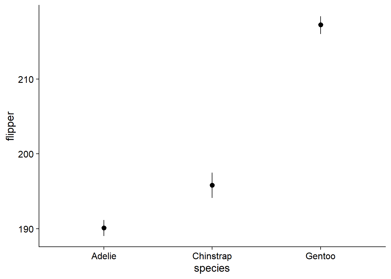
Add Mean and 95% CI
You could always just plot the mean and 95% CI (confidence intervals) and nothing else. However, like barplots, this comes at the cost of omitting the range and shape of your data. We will use geom_pointrange() because it easily accepts data from an external summary dataframe:
- You can also customize
geom_pointrange(), for example, withfatten = 2, size = .4 - Alternative: We can also use
stat_summary(fun.data = "mean_cl_normal"). Does not require external dataframe, but I think creating summary data is good practice, and future-proofs this procedure for ANCOVAs.
canvas + # this is our previously-defined canvas object, it passes the appropriate variables and theme
  # This function puts out the dot-whisker for the mean + 95% CI
    geom_pointrange(data = flipper_summary, # our externally-defined summary dataframe
                  aes(x = species,  # our independent variable
                      y = mean, # our outcome/dependent variable
                      ymin = loci,  # lower-bound confidence interval
                      ymax = upci # upper-bound confidence interval
                      ))
Adding Density Slab
Density and violin plots are based on kernel density, basically, a smoothed histogram of the data. Here, we add a density slab with ggdist::stat_slab():
canvas  +
  # density slab
  ggdist::stat_slab() + # add a density slab
  geom_pointrange(data = flipper_summary, # our externally-defined summary dataframe
                  aes(x = species,  # our independent variable
                      y = mean, # our outcome/dependent variable
                      ymin = loci,  # lower-bound confidence interval
                      ymax = upci # upper-bound confidence interval
                  ))
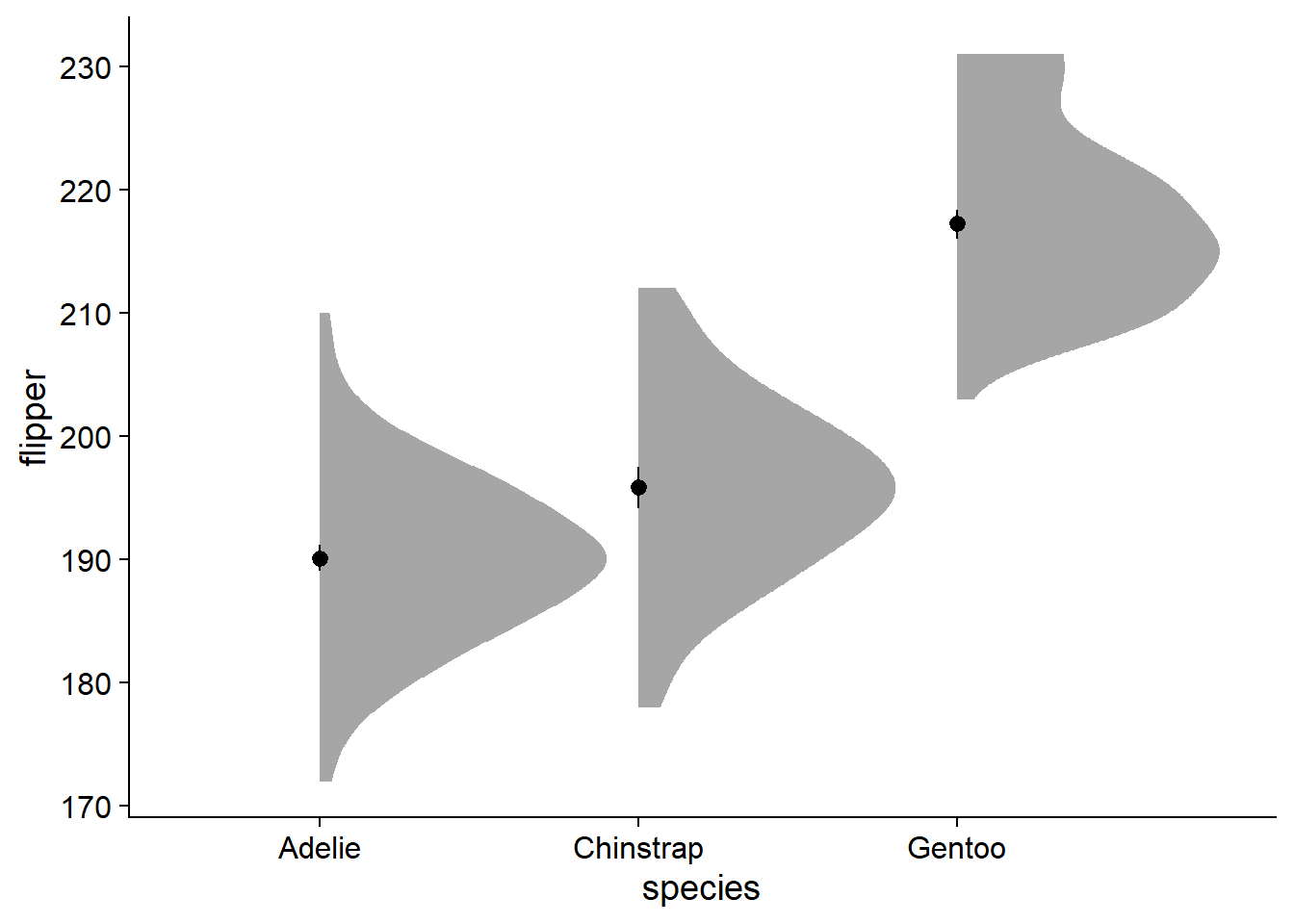
You can see the y-axis stretches far higher and lower (170 - 230) than it did previously (190 - ~210). The major strength of this density slab method is that it visualizes the spread and skew of the data, which by default forces us to visualize the entire range of observations.
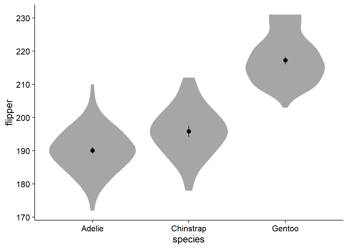
Perusing twitter conversations, some people do not like the aesthetic of a ‘lopsided’ density slab. On a more practical side, it becomes a bit more tricky to add elements like text for the mean in a legible way. To add some symmetry, we can change the density slab to violin using ggdist::stat_slab(side = "both"):
canvas +
  # density slab
  ggdist::stat_slab(
    side = "both") + # change the density slab to violin
  geom_pointrange(data = flipper_summary, # our externally-defined summary dataframe
                  aes(x = species,  # our independent variable
                      y = mean, # our outcome/dependent variable
                      ymin = loci,  # lower-bound confidence interval
                      ymax = upci # upper-bound confidence interval
                  ))
Fade and Style the Violin Plot
Many of us want to pick nice colors for our plots, in R, colors are defined with HEX codes (in this case, nova_palette[1] is #78AAA9).
You can find a generator for colorblind-accessible color palettes here, a useful tool for exploring HEX colors, complete with colorblindness simulator at the bottom of the page here, and a brief education primer, complete with colorblindness palette simulator, here.
Now we can color the violin geom with our desired Hex using fill. Notably, this only works when the fill argument is not inside of aes():
canvas +
  # density slab
  ggdist::stat_slab(side = "both",
                    fill = nova_palette[1]) + # color the violin geom with desired color
  geom_pointrange(data = flipper_summary, # our externally-defined summary dataframe
                  aes(x = species,  # our independent variable
                      y = mean, # our outcome/dependent variable
                      ymin = loci,  # lower-bound confidence interval
                      ymax = upci # upper-bound confidence interval
                  ))
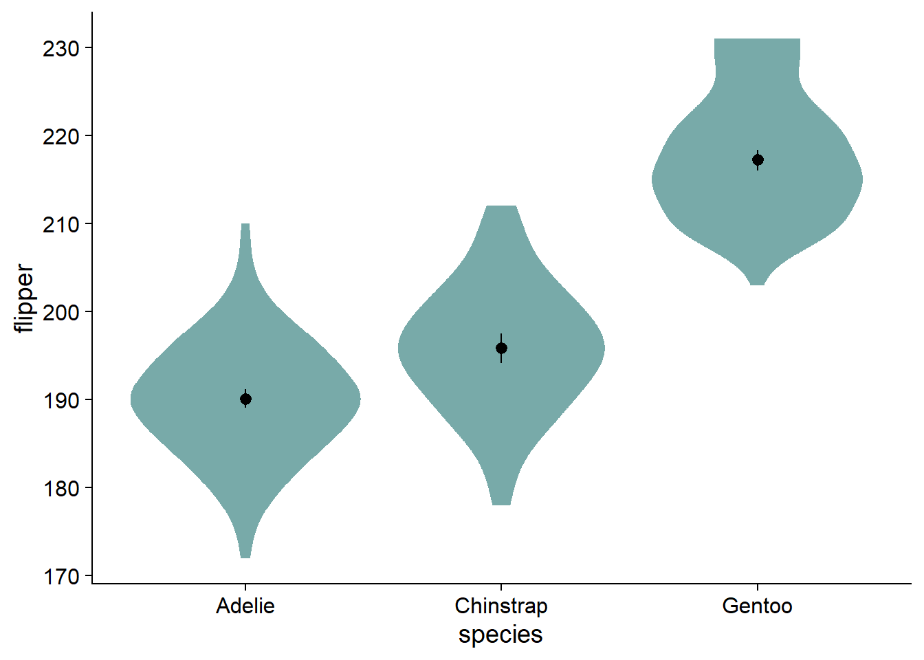
Instead of using boxplots, I like to fade my violins according to their quantile grouping. I find it makes the violin more informative, and has less visual clutter compared to the boxplot. We add the fading by modifying ggdist::stat_slab() with the argument, fill_ramp = stat(level):
canvas +
  # density slab
  ggdist::stat_slab(side = "both",
                    fill = nova_palette[1],
                    aes(fill_ramp = stat(level))) +  # fade violins according to their quantile grouping
  geom_pointrange(data = flipper_summary, # our externally-defined summary dataframe
                  aes(x = species,  # our independent variable
                      y = mean, # our outcome/dependent variable
                      ymin = loci,  # lower-bound confidence interval
                      ymax = upci # upper-bound confidence interval
                  ))
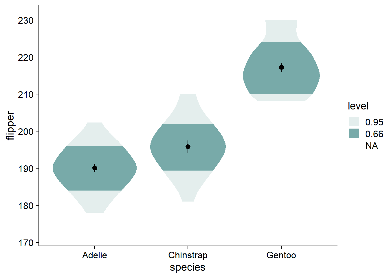
You can see by the legend that the fading matches to the inner 66% of the data, then the inner 95%, with no fading at the outer 5%. The inner 66% of the data holds no special meaning to me. I find that the inner/outer 50% is more intuitive, and directly translates to the commonly-used boxplot.
- Alternative: change from 66% to 68%, reflecting +/-1 standard deviation, giving a more direct parallel to a critical descriptive statistic (as well as cohen’s d).
We can change the shaded quantiles from the inner 66% to 50% (and eliminate the 95% shading) using ggdist::stat_slab(..., .width = c(.50, 1)):
canvas +
  # density slab
  ggdist::stat_slab(side = "both",
                    aes(fill_ramp = stat(level)),
                    fill = nova_palette[1],
                    .width = c(.50, 1)) +  # change quantiles for shading from 66% to 50% (and eliminate the 95% shading)
  geom_pointrange(data = flipper_summary, # our externally-defined summary dataframe
                  aes(x = species,  # our independent variable
                      y = mean, # our outcome/dependent variable
                      ymin = loci,  # lower-bound confidence interval
                      ymax = upci # upper-bound confidence interval
                  ))
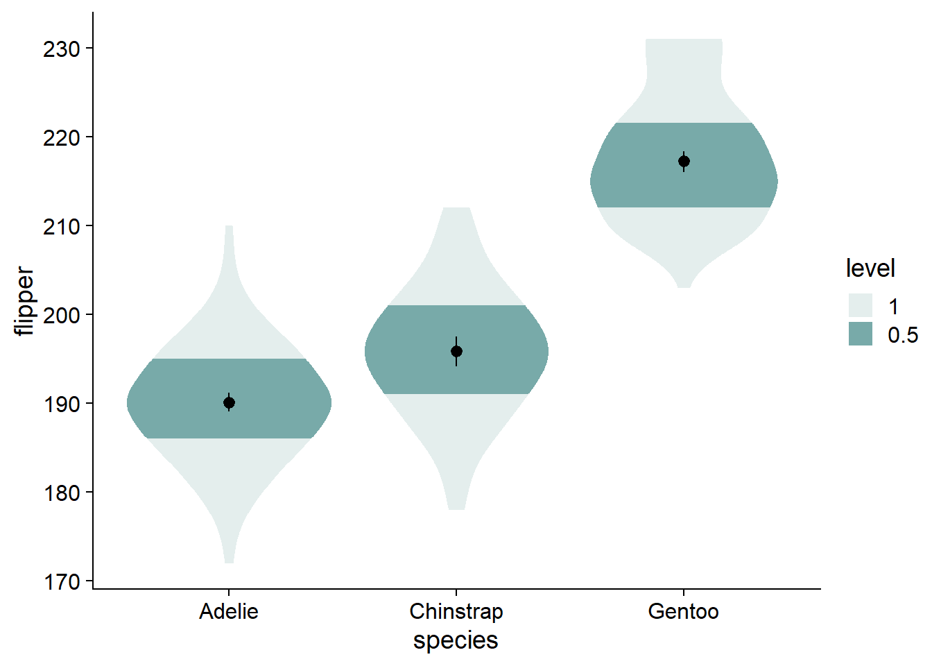
The violins are quite wide, let’s adjust their widths using scale = .4.
canvas +
  # density slab
  ggdist::stat_slab(side = "both",
                    aes(fill_ramp = stat(level)),
                    fill = nova_palette[1],
                    .width = c(.50, 1),
                    scale = .4) +  # adjust slab width
  geom_pointrange(data = flipper_summary, # our externally-defined summary dataframe
                  aes(x = species,  # our independent variable
                      y = mean, # our outcome/dependent variable
                      ymin = loci,  # lower-bound confidence interval
                      ymax = upci # upper-bound confidence interval
                  ))
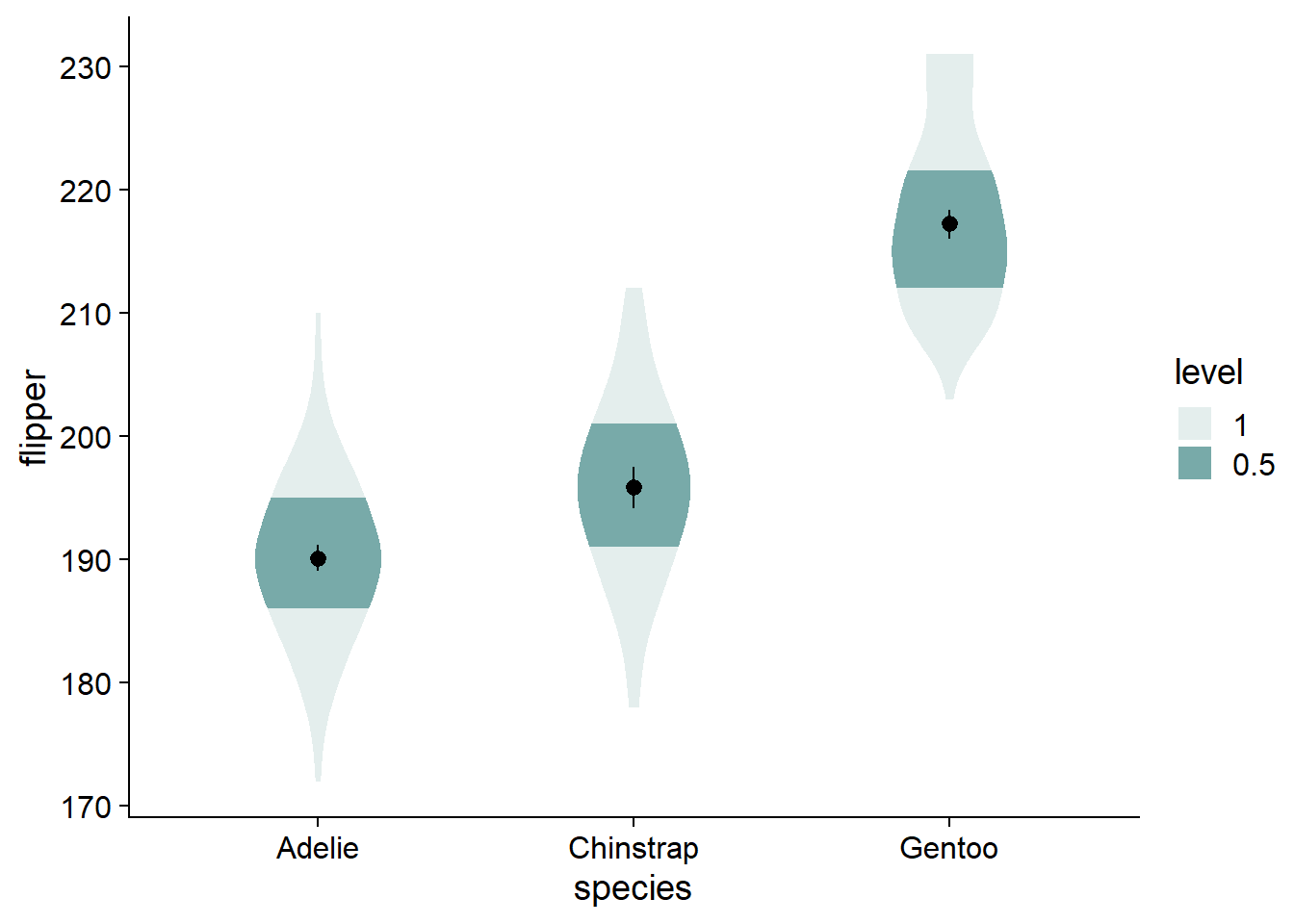
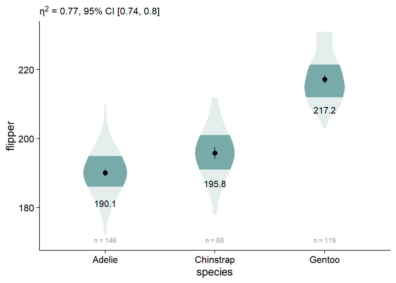
The fading quantiles are probably better discussed orally or as a figure note, not being directly relevant to any statistical tests. We can get rid of the legend element for fading quantiles with guides(fill_ramp = "none"). Here, we also assign this ggplot to a new object, viofade, so we can see new code additions in the chunks more easily:
viofade <- canvas +
  # density slab
  ggdist::stat_slab(side = "both",
                    aes(fill_ramp = stat(level)),
                    fill = nova_palette[1],
                    .width = c(.50, 1),
                    scale = .4) +
  geom_pointrange(data = flipper_summary, # our externally-defined summary dataframe
                  aes(x = species,  # our independent variable
                      y = mean, # our outcome/dependent variable
                      ymin = loci,  # lower-bound confidence interval
                      ymax = upci # upper-bound confidence interval
                  ))  +
  guides(fill_ramp = "none") # get rid of legend element for fading quantiles

viofade
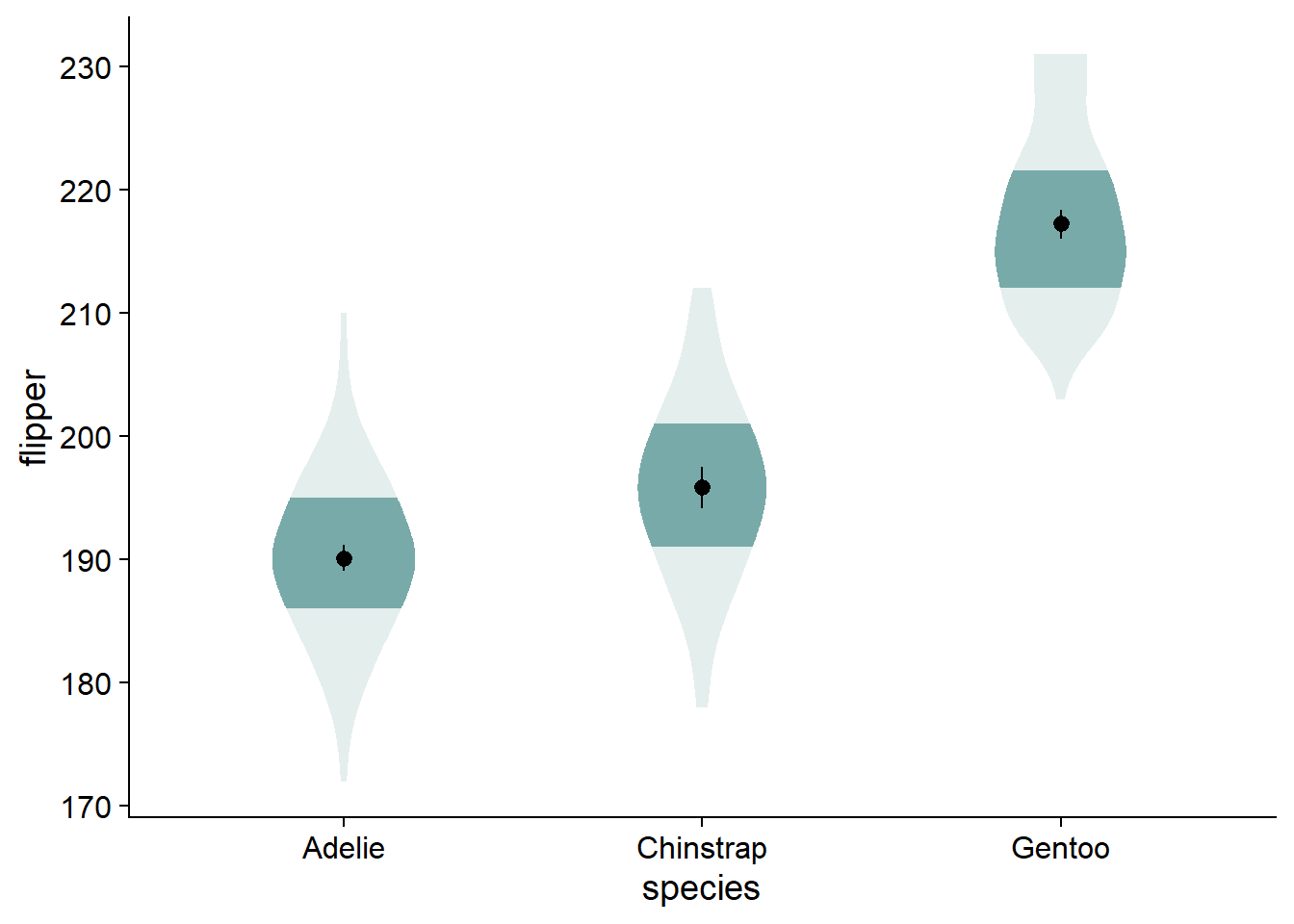
This is a satisfactory version of the complete viofade, but like any makeover, there is more styling we can do.
Adding Extra Elements
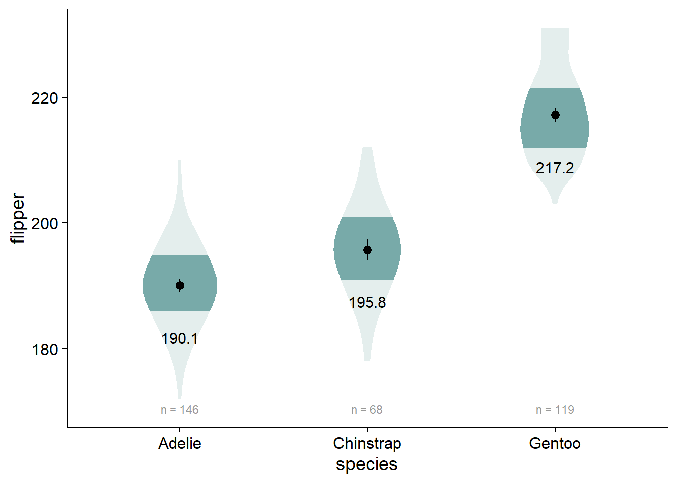
I find that having the written values of the different means makes the comparisons a bit more concrete. Again, you could use stat_summary(), but we will keep using our flipper_summary data, this time with geom_text().
viofade +
  geom_text(data = flipper_summary,
            aes(x = species,
                y = mean,
                label = round(mean,1)),
            color="black",
            size = 4,
            vjust = 5)

# You could use this function if you want:
   # stat_summary(aes(label = round(..y..,1)),
   #                         fun = mean,
   #                         geom = "text",vjust = 5)
Our viofade object does not include raw data. This is intentional because objects such as rainclouds, fadeclouds, and shadeplots tend to look very noisy after I add significance brackets. However, I still want people to see the sample size for our groups, which we can do using geom_text() in combination with our flipper_summary dataframe.
- Alternative: Use
EnvStats::stat_n_text()if you don’t want to use a summary dataframe, although I don’t think this method works with a factorial design (i.e., you can’t “dodge” the positions of these elements) - If you want your sample sizes under your axis values, check out this discussion
viofade_text <- viofade +
  geom_text(data = flipper_summary, aes(x = species,
                                        y = mean,
                                        label = round(mean,1)),
            color="black",
            size = 4,
            vjust = 5) +
  geom_text(data = flipper_summary,
            aes(label = paste("n =", n),
                y = flipper_summary[which.min(flipper_summary$min),]$mean -
                  3*flipper_summary[which.min(flipper_summary$min),]$std_dev), #  dynamically set the location of sample size (3 standard deviations below the mean of the lowest-scoring group)
            size = 3,
            color = "grey60")

# You could use this for sample sizes if you want
 # EnvStats::stat_n_text(color = "grey60")

viofade_text
Adding Test Statistics
Especially for presentations and posters, it can be useful to have significance tests embedded directly in the plot. This is where we really benefit from having run some analyses beforehand.
Using our pre-run analyses is made much easier if we write a helper function, so here we create a custom function, report_tidy_anova_etaci() that facilitate reporting of significance and effect size statistics for our ANOVA (for eta squared).
Click here if you want to see the script `report_tidy_anova_etaci()`!
# This function generates a text summary of ANOVA results based on user-specified options.
report_tidy_anova_etaci <- function(tidy_frame, # Your tidy ANOVA dataframe
                                    term, # The predictor in your tidy ANOVA dataframe
                                    effsize = TRUE, # Display the effect size
                                    ci95 = TRUE, # Display the 95% CI
                                    ci.lab = TRUE, # Display the "95% CI" label
                                    teststat = TRUE, # Display the F-score and degrees of freedom
                                    pval = TRUE # Display the p-value
                                    ){
  # Initialize an empty string to store the result text
  text <- ""

  # Conditionally add effect size (eta square) to the result text
  if (effsize == TRUE) {
    text <- paste0(text,
      "\u03b7^2^ = ", # Unicode for eta square
      round(as.numeric(tidy_frame[term, "pes"]), 2)
    )
  }

  # Conditionally add 95% CI to the result text
  if (ci95 == TRUE) {
    text <- paste0(text,
      ifelse(ci.lab == TRUE,
        paste0(", 95% CI ["), " ["),
      round(as.numeric(tidy_frame[term, "pes_ci95_lo"]), 2), ", ",
      round(as.numeric(tidy_frame[term, "pes_ci95_hi"]), 2), "]"
    )
  }

  # Conditionally add F-score and degrees of freedom to the result text
  if (teststat == TRUE) {
    text <- paste0(text,
      ", *F*(", tidy_frame[term, "Df"],
      ", ", tidy_frame["Residuals", "Df"], ") = ",
      round(as.numeric(tidy_frame[term, "F.value"], 2))
    )
  }

  # Conditionally add p-value to the result text
  if (pval == TRUE) {
    text <- paste0(text,
      ", ",  report_pval_full(tidy_frame[term, "Pr..F."])
    )
  }

  # Return the generated text summary
  return(text)
}
We can add our omnibus ANOVA test by embedding our custom function in the labs element, labs(subtitle = report_tidy_anova_etaci(flipper_anova,"species")):
viofade_text +
  labs(subtitle = report_tidy_anova_etaci(flipper_anova,"species"))
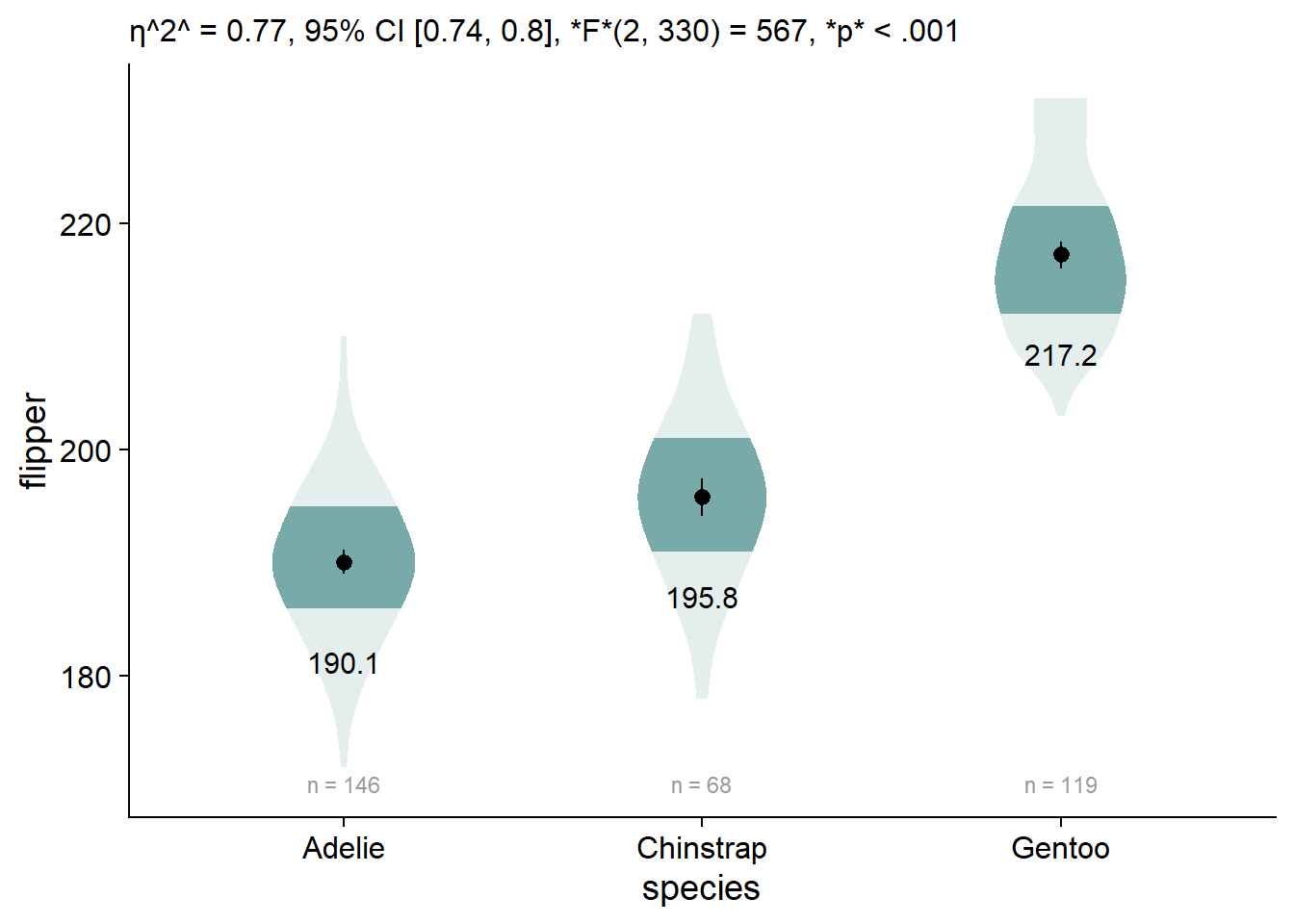
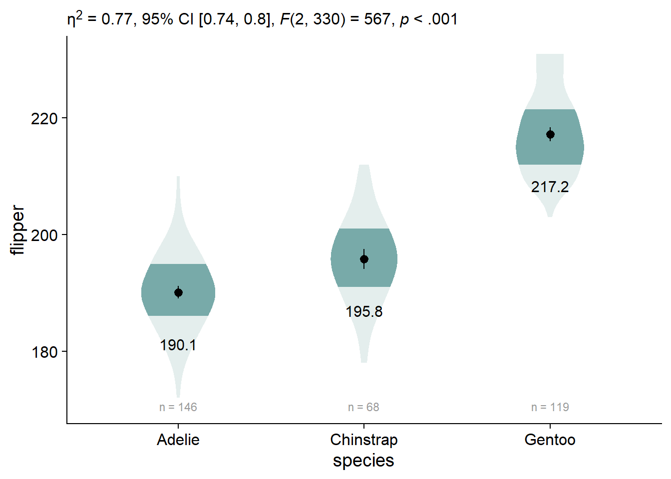
By default, ggplot doesn’t allow markdown styling, so we have weird stars instead of our desired formatting. We can enable markdown styling in the subtitle by using theme(plot.subtitle = ggtext::element_markdown()):
viofade_text_stats <- viofade_text +
  labs(subtitle = report_tidy_anova_etaci(flipper_anova,"species")) +
  theme(plot.subtitle = ggtext::element_markdown())

viofade_text_stats
We can also customize our anova extraction function, report_tidy_anova_etaci() to show less information in the subtitle.
viofade_text +
  labs(subtitle = report_tidy_anova_etaci(flipper_anova,
                                          "species",
                                          teststat = FALSE,
                                          pval = FALSE)) +
  theme(plot.subtitle = ggtext::element_markdown())
Add Significance Brackets
Adding significance brackets using the function ggpubr::geom_bracket(), and our previously-defined object flipper_emmeans_contrasts. You’ll have to manually select and place the appropriate contrast.
viofade_text_stats_bracket1 <- viofade_text_stats +
  ggpubr::geom_bracket(
                       tip.length = 0.02, # the downard "tips" of the bracket
                       vjust = 0, # moves your text label (in this case, the p-value)
                       xmin = 1, #starting point for the bracket
                       xmax = 2, # ending point for the bracket
                       y.position = 220, # vertical location of the bracket
                       label.size = 2.5, # size of your bracket text
                       label = paste0(
                         report_tidy_t(
                           flipper_emmeans_contrasts[flipper_emmeans_contrasts$contrast =="Adelie - Chinstrap",],
                           italicize = FALSE,
                           ci = FALSE)) # content of your bracket text
  )

viofade_text_stats_bracket1

You can also add some additional text to the labels for your significance brackets using ggpubr::geom_bracket(..., label = paste0(...))
viofade_text_stats_bracket2 <- viofade_text_stats_bracket1 +
  ggpubr::geom_bracket(
    tip.length = 0.02,
    vjust = 0,
    xmin = 2,
    xmax = 3,
    y.position = 227 ,
    label.size = 2.5,
    label = paste0("My hypothesis, ",
                   report_tidy_t(flipper_emmeans_contrasts[flipper_emmeans_contrasts$contrast =="Adelie - Chinstrap",],
                                 italicize = FALSE,
                                 ci = FALSE,
                                 point = FALSE,
                                 pval_comma= FALSE))
  )
Style on the axis titles with theme(), ylab(), and xlab()
viofade_text_stats_bracket2 +
  theme(axis.title = element_text(face="bold")) +
  ylab("Flipper length (mm)") +
  xlab("Species")

Click Here to see comparisons to alternatives, like the shadeplot, fadecloud, and faded dotplot

dark_aqua <- "#1E716F"
fresh_canvas <- canvas +
theme(axis.title = element_text(face="bold")) +
ylab("Flipper length (mm)") +
xlab("Species") +
geom_text(data = flipper_summary,
aes(label = paste("n =", n),
y = flipper_summary[which.min(flipper_summary$min),]$mean -
3.2*flipper_summary[which.min(flipper_summary$min),]$std_dev), # dynamically set the location of sample size (3 standard deviations below the mean of the lowest-scoring group)
size = 2.5,
color = "grey60")
dotwhisker <- geom_pointrange(data = flipper_summary,
aes(x = species,
mean,
ymin = loci,
ymax = upci),
# fatten = 2,
size = .5,
position = ggpp::position_dodge2nudge(x = -.07),
color = "black",
show.legend = FALSE)
# add mean text
meantext <- geom_text(data = flipper_summary,
aes(x = species,
y = mean,
label = round(mean,1)),
color="black", size = 3.2,
position = ggpp::position_dodge2nudge(x = -.25))
offset_bracket1 <- ggpubr::geom_bracket(
tip.length = 0.02, # the downard "tips" of the bracket
vjust = 0, # moves your text label (in this case, the p-value)
xmin = .93, #starting point for the bracket
xmax = 1.93, # ending point for the bracket
y.position = 220, # vertical location of the bracket
label.size = 2.5, # size of your bracket text
label = paste0("My hypothesis, ",
report_tidy_t(flipper_emmeans_contrasts[flipper_emmeans_contrasts$contrast =="Adelie - Chinstrap",],
italicize = FALSE,
ci = FALSE,
point = FALSE,
pval_comma= FALSE)) # content of your bracket text
)
offset_bracket2 <- ggpubr::geom_bracket(
tip.length = 0.02,
vjust = 0,
xmin = 1.93,
xmax = 2.93,
y.position = 227 ,
label.size = 2.5,
label = paste0("My hypothesis, ",
report_tidy_t(flipper_emmeans_contrasts[flipper_emmeans_contrasts$contrast == "Chinstrap - Gentoo",],
italicize = FALSE,
ci = FALSE,
point = FALSE,
pval_comma= FALSE)))
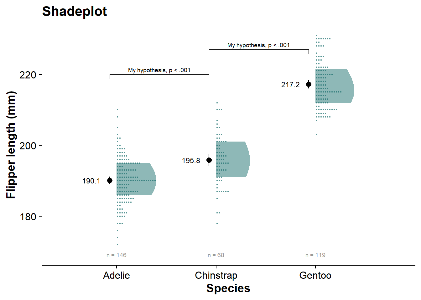
shadeplot <- fresh_canvas +
## Add density slab
ggdist::stat_slab( alpha = 0.5,
adjust = 2,
side = "right",
scale = 0.4,
show.legend = F,
position = position_dodge(width = .8),
.width = c(.50, 1),
fill = dark_aqua,
aes(fill_ramp = stat(level))) +
## Add stacked dots
ggdist::stat_dots(alpha = 0.5,
side = "right",
scale = 0.4,
color = dark_aqua,
fill = dark_aqua,
# dotsize = 1.5,
position = position_dodge(width = .8)) +
ggdist::scale_fill_ramp_discrete(range = c(0.0, 1),
aesthetics = c("fill_ramp")) +
dotwhisker +
meantext +
offset_bracket1 +
offset_bracket2 +
labs(title = "Shadeplot")
shadeplot
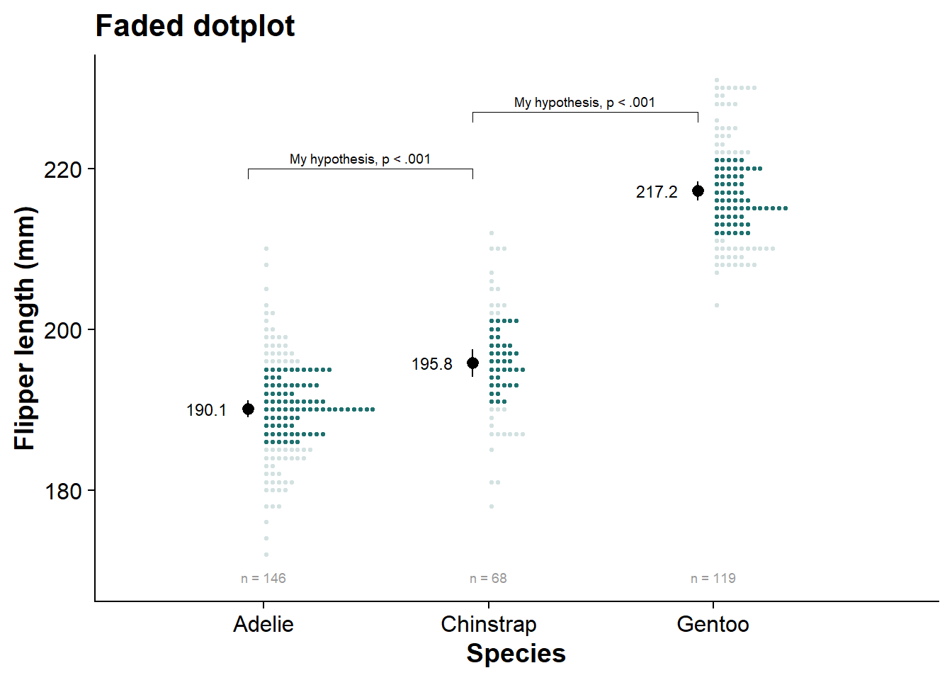
faded_dotplot <- fresh_canvas +
  ggdist::stat_dots(side = "right", ## set direction of dots
                    scale = 0.5, ## defines the highest level the dots can be stacked to
                    show.legend = F,
                    dotsize = 1.5,
                    position = position_dodge(width = .8),
                    ## stat- and colour-related properties
                    .width = c(.50, 1), ## set quantiles for shading
                    aes(colour_ramp = stat(level), ## set stat ramping and assign colour/fill to variable
                        fill_ramp = stat(level)),
                    color = dark_aqua,
                    fill = dark_aqua)  +
  dotwhisker +
  meantext +
  offset_bracket1 +
  offset_bracket2  +
  labs(title = "Faded dotplot")

faded_dotplot
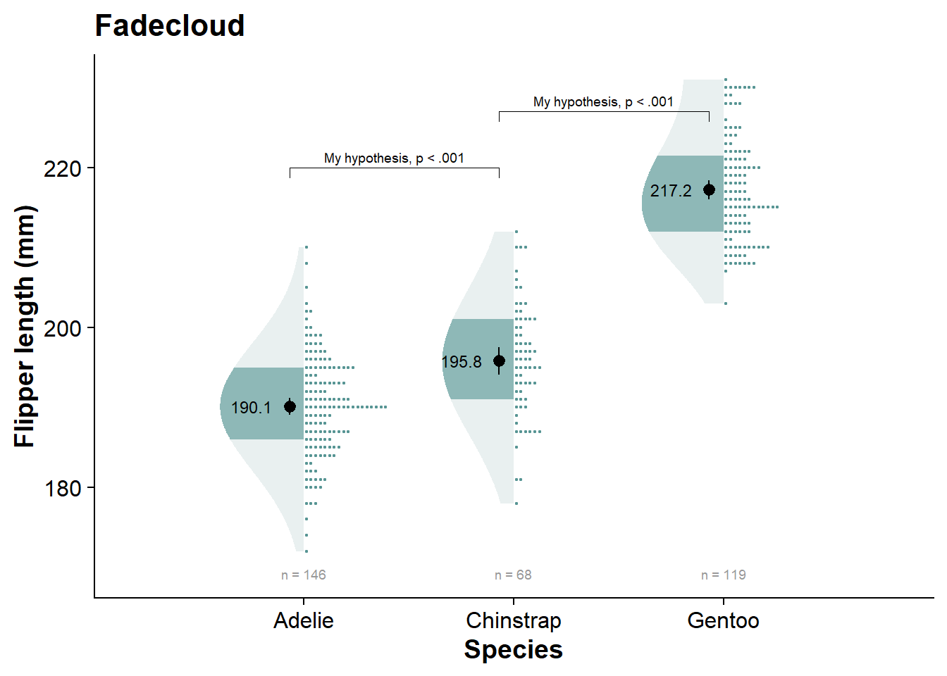
fadecloud <- fresh_canvas +
  ggdist::stat_slab( alpha = 0.5,
                     adjust = 2,
                     side = "left",
                     scale = 0.4,
                     show.legend = F,
                     position = position_dodge(width = .8),
                     .width = c(.50, 1),
                     fill = dark_aqua,
                     aes(fill_ramp = stat(level))) +
  ## dots
  ggdist::stat_dots(alpha = 0.5,
                    side = "right",
                    scale = 0.4,
                    color = dark_aqua,
                    fill = dark_aqua,
                    # dotsize = 1.5,
                    position = position_dodge(width = .8)) +
  dotwhisker +
  meantext +
  offset_bracket1 +
  offset_bracket2 +
  labs(title = "Fadecloud")

fadecloud
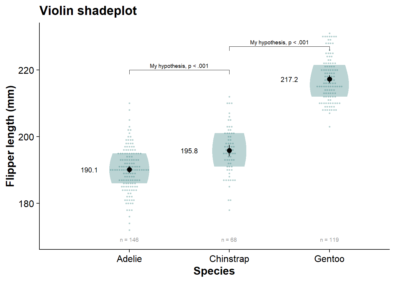
vioshadeplot <- fresh_canvas +
  ggdist::stat_slab( alpha = .5,
                     adjust = 2,
                     side = "both",
                     scale = 0.4,
                     show.legend = F,
                     position = position_dodge(width = .8),
                     .width = c(.50, 1),
                     fill = nova_palette[1],
                     aes(fill_ramp = stat(level))) +
  ## Add stacked dots
  ggdist::stat_dots(alpha = 0.2,
                    side = "both",
                    scale = 0.4,
                    color = dark_aqua,
                    fill = dark_aqua,
                    # dotsize = 1.5,
                    position = position_dodge(width = .8)) +
  ggdist::scale_fill_ramp_discrete(range = c(0.0, 1),
                                   aesthetics = c("fill_ramp")) +
  geom_pointrange(data = flipper_summary,
                  aes(x = species,
                      mean,
                      ymin = loci,
                      ymax = upci),
                  size = .5,
                  color = "black",
                  show.legend = FALSE) +
  # add mean text
  geom_text(data = flipper_summary,
            aes(x = species,
                y = mean,
                label = round(mean,1)),
            color="black", size = 3.2,
            position = ggpp::position_dodge2nudge(x = -.4)) +
  ggpubr::geom_bracket(
    tip.length = 0.02, # the downard "tips" of the bracket
    vjust = 0, # moves your text label (in this case, the p-value)
    xmin = 1, #starting point for the bracket
    xmax = 2, # ending point for the bracket
    y.position = 220, # vertical location of the bracket
    label.size = 2.5, # size of your bracket text
    label = paste0("My hypothesis, ",
                   report_tidy_t(flipper_emmeans_contrasts[flipper_emmeans_contrasts$contrast =="Adelie - Chinstrap",],
                                 italicize = FALSE,
                                 ci = FALSE,
                                 point = FALSE,
                                 pval_comma= FALSE))
  ) +
  ggpubr::geom_bracket(
    tip.length = 0.02,
    vjust = 0,
    xmin = 2,
    xmax = 3,
    y.position = 227 ,
    label.size = 2.5,
    label = paste0("My hypothesis, ",
                   report_tidy_t(flipper_emmeans_contrasts[flipper_emmeans_contrasts$contrast =="Chinstrap - Gentoo",],
                                 italicize = FALSE,
                                 ci = FALSE,
                                 point = FALSE,
                                 pval_comma= FALSE))
  ) +
  labs(title = "Violin shadeplot")


vioshadeplot
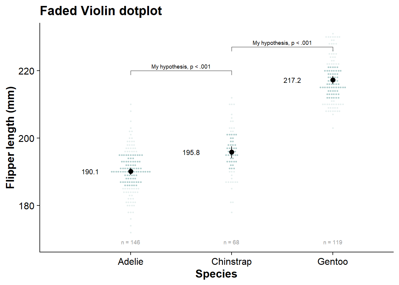
viofade_dotplot <- fresh_canvas +
  ggdist::stat_dots(side = "both", ## set direction of dots
                    scale = 0.4, ## defines the highest level the dots can be stacked to
                    alpha = .4,
                    show.legend = F,
                    dotsize = 1.5,
                    position = position_dodge(width = .8),
                    ## stat- and colour-related properties
                    .width = c(.50, 1), ## set quantiles for shading
                    aes(colour_ramp = stat(level), ## set stat ramping and assign colour/fill to variable
                        fill_ramp = stat(level)),
                    color = nova_palette[1],
                    fill = nova_palette[1])  +
  ggdist::scale_fill_ramp_discrete(range = c(0.5, 1),
                                   aesthetics = c("fill_ramp")) +
  geom_pointrange(data = flipper_summary,
                  aes(x = species,
                      mean,
                      ymin = loci,
                      ymax = upci),
                  size = .5,
                  color = "black",
                  show.legend = FALSE) +
  # add mean text
  geom_text(data = flipper_summary,
            aes(x = species,
                y = mean,
                label = round(mean,1)),
            color="black",
            size = 3.2,
            position = ggpp::position_dodge2nudge(x = -.4)) +
  ggpubr::geom_bracket(
    tip.length = 0.02, # the downard "tips" of the bracket
    vjust = 0, # moves your text label (in this case, the p-value)
    xmin = 1, #starting point for the bracket
    xmax = 2, # ending point for the bracket
    y.position = 220, # vertical location of the bracket
    label.size = 2.5, # size of your bracket text
    label = paste0("My hypothesis, ",
                   report_tidy_t(flipper_emmeans_contrasts[flipper_emmeans_contrasts$contrast =="Adelie - Chinstrap",],
                                 italicize = FALSE,
                                 ci = FALSE,
                                 point = FALSE,
                                 pval_comma= FALSE)) # content of your bracket text
  ) +
  ggpubr::geom_bracket(
    tip.length = 0.02,
    vjust = 0,
    xmin = 2,
    xmax = 3,
    y.position = 227 ,
    label.size = 2.5,
    label = paste0("My hypothesis, ",
                   report_tidy_t(flipper_emmeans_contrasts[flipper_emmeans_contrasts$contrast =="Chinstrap - Gentoo",],
                                 italicize = FALSE,
                                 ci = FALSE,
                                 point = FALSE,
                                 pval_comma= FALSE))
  ) +
  labs(title = "Faded Violin dotplot")

viofade_dotplot
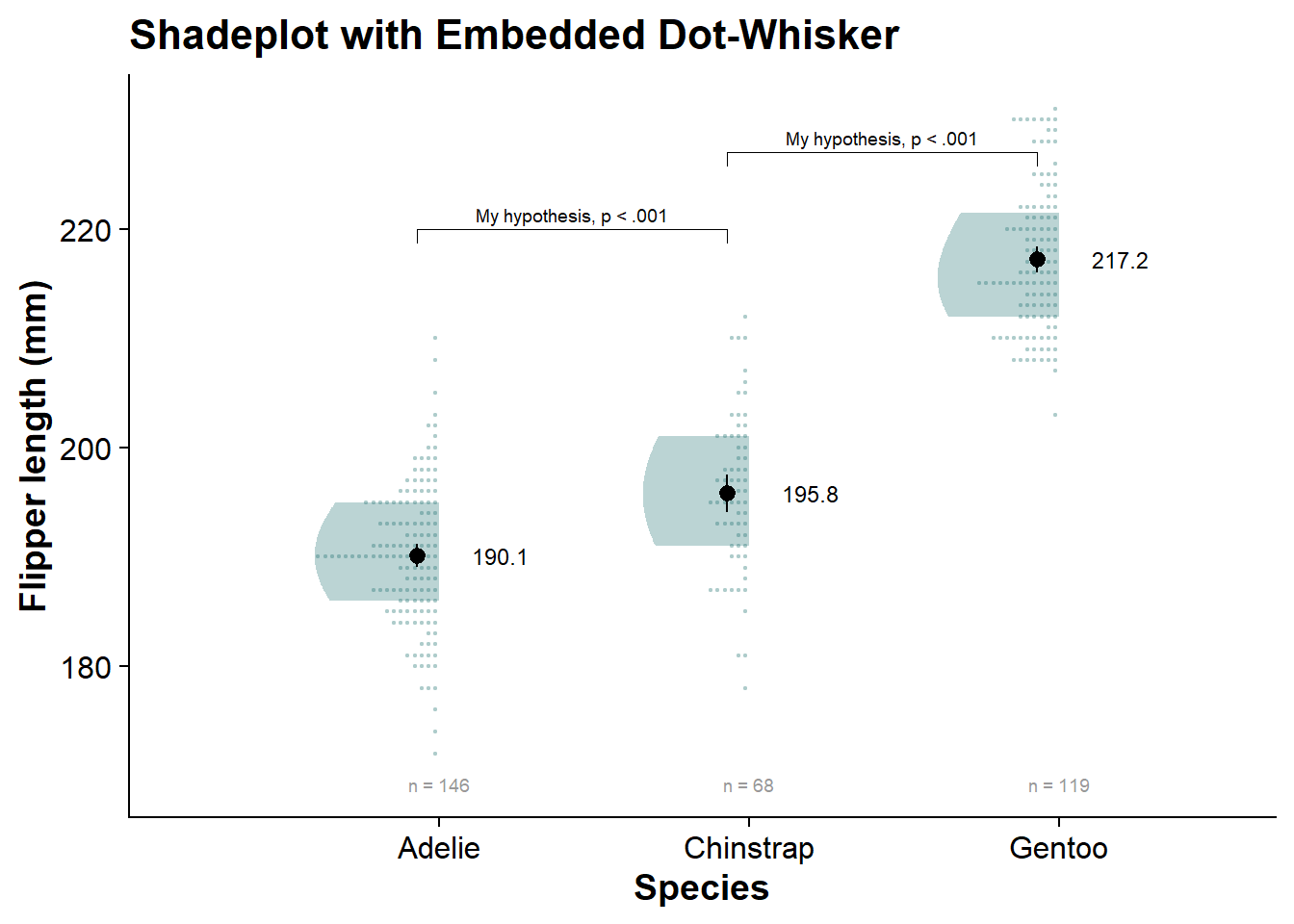
internal_shadeplot <- fresh_canvas +
  ## Add density slab
  ggdist::stat_slab( alpha = .5,
                     adjust = 2,
                     side = "left",
                     scale = 0.4,
                     show.legend = F,
                     position = position_dodge(width = .8),
                     .width = c(.50, 1),
                     fill = nova_palette[1],
                     aes(fill_ramp = stat(level))) +
  ## Add stacked dots
  ggdist::stat_dots(alpha = 0.2,
                    side = "left",
                    scale = 0.4,
                    color = dark_aqua,
                    fill = dark_aqua,
                    # dotsize = 1.5,
                    position = position_dodge(width = .8)) +
  ggdist::scale_fill_ramp_discrete(range = c(0.0, 1),
                                   aesthetics = c("fill_ramp")) +
  geom_pointrange(data = flipper_summary,
                  aes(x = species,
                      mean,
                      ymin = loci,
                      ymax = upci),
                  size = .5,
                  color = "black",
                  position = ggpp::position_dodge2nudge(x = -.07),
                  show.legend = FALSE) +
  # add mean text
  geom_text(data = flipper_summary,
            aes(x = species,
                y = mean,
                label = round(mean,1)),
            color="black", size = 3.2,
            position = ggpp::position_dodge2nudge(x = .2)) +

  offset_bracket1 +
  offset_bracket2 +
  labs(title = "Shadeplot with Embedded Dot-Whisker")


internal_shadeplot
Saving Your Plot
A final step in the reproducible pipeline is to automate the saving of your up-to-date graph. You can do this with ggsave() for your most recently-created plot.
Also, see a basic guide here, the tidyverse guide here, a guide hilighting more saving options here, a detailed guide here, and a video here
# save your most recently-displayed plot in a folder called "figures"
ggsave(here::here("figures", "viofade.png"),
       width=7, height = 5, dpi=700)
Now Try a Factorial Design
Nicely-designed code and workflows can often break down in even slightly new use cases. For my purposes, I often run factorial designs (plotting multiple independent variables at once). Now we can show how this workflow incorporates this type of analysis:
Summarize the Factorial Data
Our data
flipper_fact_summary <- make_summary(data = df, dv = flipper, grouping1 = species, grouping2 = sex)

knitr::kable(flipper_fact_summary)
| species | sex | mean | min | max | n | std_dev | se | y25 | y50 | y75 | loci | upci |
|---|---|---|---|---|---|---|---|---|---|---|---|---|
| Adelie | female | 187.79 | 172 | 202 | 73 | 5.60 | 0.65 | 185 | 188 | 191 | 186.5260 | 189.0740 |
| Adelie | male | 192.41 | 178 | 210 | 73 | 6.60 | 0.77 | 189 | 193 | 197 | 190.8908 | 193.9092 |
| Chinstrap | female | 191.74 | 178 | 202 | 34 | 5.75 | 0.99 | 187 | 192 | 196 | 189.7596 | 193.6404 |
| Chinstrap | male | 199.91 | 187 | 212 | 34 | 5.98 | 1.02 | 196 | 200 | 203 | 197.9008 | 201.8992 |
| Gentoo | female | 212.71 | 203 | 222 | 58 | 3.90 | 0.51 | 210 | 212 | 215 | 211.7004 | 213.6996 |
| Gentoo | male | 221.54 | 208 | 231 | 61 | 5.67 | 0.73 | 218 | 221 | 225 | 220.0692 | 222.9308 |
Analyze the Factorial Data
# Fit data
flipper_fact_fit <- stats::aov(flipper ~ species*sex, data = df)
# Run anova
flipper_fact_anova <- car::Anova(flipper_fact_fit,
                                 type=3
                                 )
Eta Square
Calculate effect sizes with effectsize::eta_squared()
flipper_fact_anova_pes <- effectsize::eta_squared(flipper_fact_anova,
                                             alternative="two.sided"
                                             )

flipper_fact_anova <- data.frame(flipper_fact_anova)
flipper_fact_anova <- flipper_fact_anova[!(rownames(flipper_fact_anova) == "(Intercept)"), ]

flipper_fact_anova[1:3,"pes_ci95_lo"] <- flipper_fact_anova_pes$CI_low
flipper_fact_anova[1:3,"pes_ci95_hi"] <- flipper_fact_anova_pes$CI_high
flipper_fact_anova[1:3,"pes"] <- flipper_fact_anova_pes$Eta2


flipper_fact_anova <- flipper_fact_anova %>%
  dplyr::mutate_if(is.numeric, function(x) round(x, 3))

knitr::kable(flipper_fact_anova)
| Sum.Sq | Df | F.value | Pr..F. | pes_ci95_lo | pes_ci95_hi | pes | |
|---|---|---|---|---|---|---|---|
| species | 50075.839 | 2 | 782.876 | 0.000 | 0.798 | 0.851 | 0.827 |
| sex | 3902.420 | 1 | 122.019 | 0.000 | 0.195 | 0.347 | 0.272 |
| species:sex | 329.042 | 2 | 5.144 | 0.006 | 0.003 | 0.073 | 0.031 |
| Residuals | 10458.107 | 327 | NA | NA | NA | NA | NA |
Estimated Marginal Means
Extract estimated marginal means with emmeans::emmeans() and merge with basic summary dataframe with our custom merge_emmeans_summary() function:
# Extract estimated marginal means
flipper_fact_emmeans <- emmeans::emmeans(flipper_fact_fit, specs = pairwise ~ species:sex)


# Convert estimated marginal means to dataframe
flipper_fact_emmeans_tidy <- data.frame(flipper_fact_emmeans$emmeans)


flipper_fact_summary <- flipper_fact_summary[order(flipper_fact_summary$species,
                                                   flipper_fact_summary$sex), ]

flipper_fact_emmeans_tidy <- flipper_fact_emmeans_tidy[order(flipper_fact_emmeans_tidy$species,
                                                             flipper_fact_emmeans_tidy$sex), ]


flipper_fact_summary <- merge_emmeans_summary(summary_data = flipper_fact_summary,
                                                  emmeans_tidy = flipper_fact_emmeans_tidy)

flipper_fact_summary <- flipper_fact_summary %>%
  mutate_if(is.numeric, function(x) round(x, 2))

knitr::kable(flipper_fact_summary)
| species | sex | mean | min | max | n | std_dev | se | y25 | y50 | y75 | loci | upci | emmean | emmean_se | emmean_loci | emmean_upci |
|---|---|---|---|---|---|---|---|---|---|---|---|---|---|---|---|---|
| Adelie | female | 187.79 | 172 | 202 | 73 | 5.60 | 0.65 | 185 | 188 | 191 | 186.53 | 189.07 | 187.79 | 0.66 | 186.49 | 189.10 |
| Adelie | male | 192.41 | 178 | 210 | 73 | 6.60 | 0.77 | 189 | 193 | 197 | 190.89 | 193.91 | 192.41 | 0.66 | 191.11 | 193.71 |
| Chinstrap | female | 191.74 | 178 | 202 | 34 | 5.75 | 0.99 | 187 | 192 | 196 | 189.76 | 193.64 | 191.74 | 0.97 | 189.83 | 193.64 |
| Chinstrap | male | 199.91 | 187 | 212 | 34 | 5.98 | 1.02 | 196 | 200 | 203 | 197.90 | 201.90 | 199.91 | 0.97 | 198.00 | 201.82 |
| Gentoo | female | 212.71 | 203 | 222 | 58 | 3.90 | 0.51 | 210 | 212 | 215 | 211.70 | 213.70 | 212.71 | 0.74 | 211.25 | 214.17 |
| Gentoo | male | 221.54 | 208 | 231 | 61 | 5.67 | 0.73 | 218 | 221 | 225 | 220.07 | 222.93 | 221.54 | 0.72 | 220.12 | 222.97 |
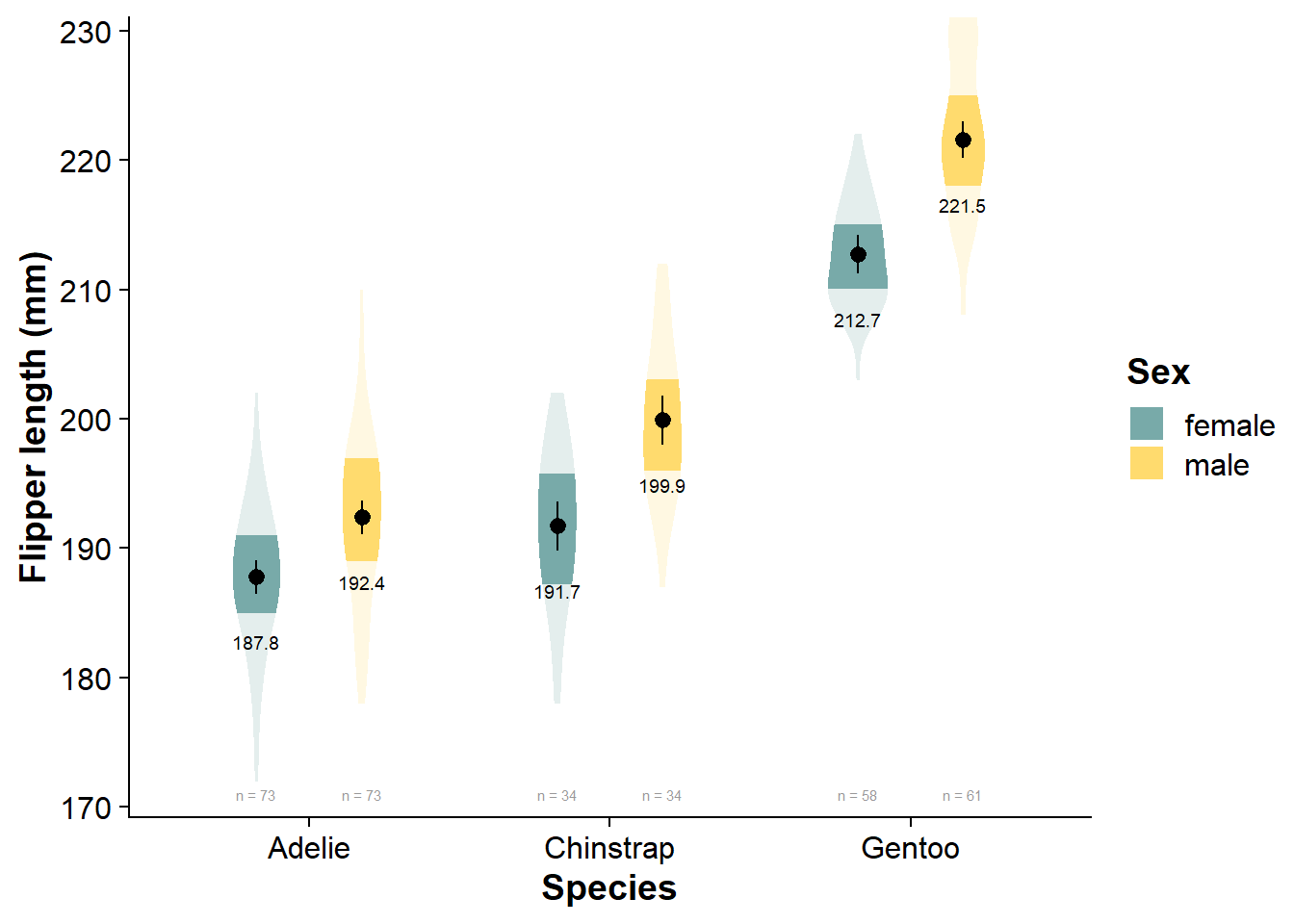
Vizualize the Factorial Data
viofade_fact <- ggplot(data = df,
                       aes(y = flipper, # our dependent/response/outcome variable
                           x = species,  # our grouping/independent/predictor variable
                           fill = sex)) +  # our third grouping/independent/interaction variable
  ggdist::stat_slab(side = "both",
                    aes(fill_ramp = stat(level)),
                    .width = c(.50, 1),
                    scale = .4,
                    position = position_dodge(width = .7)) +
  scale_fill_manual(values = nova_palette) +
  # stat_summary(fun.data = "mean_cl_normal",
  #              show.legend = F,
  #              color = "black",
  #              position = position_dodge(width = .7))  +
  geom_pointrange(data = flipper_fact_summary,
                  aes(x = species,
                      y = emmean,
                      ymin = emmean_loci,
                      ymax = emmean_upci),
                  position = position_dodge(.7), show.legend = F) +
  geom_text(data = flipper_fact_summary, aes(x = species,
                                             y = emmean,
                                             label = round(emmean,1)),
            color="black",
            size = 2.5,
            vjust = 5,
            position = position_dodge(width = .7)) +
  # stat_summary(aes(label=round(..y..,0)),
  #              fun=mean, geom="text",
  #              position = position_dodge(width = .7),
  #              size=2.5,
  #              vjust = 5) +
  geom_text(data = flipper_fact_summary,
            aes(label = paste("n =", n),
                y = flipper_fact_summary[which.min(flipper_fact_summary$min),]$mean -
                  3*flipper_fact_summary[which.min(flipper_fact_summary$min),]$std_dev), #  dynamically set the location of sample size (3 standard deviations below the mean of the lowest-scoring group)
            size = 2,
            color = "grey60",
            position = position_dodge(width = .7)) +
  guides(fill_ramp = "none") +
  scale_y_continuous(expand = expansion(mult = c(0.03, 0))) +
  cowplot::theme_half_open() +
  theme(axis.title = element_text(face="bold"),
        legend.title = element_text(face="bold")) +
  labs(x = "Species",
       y = "Flipper length (mm)",
       fill = "Sex")


viofade_fact
Pairwise Comparisons
# convert estimated marginal mean contrasts to dataframe
flipper_fact_emmeans_contrasts <- data.frame(flipper_fact_emmeans$contrasts)

flipper_fact_emmeans_contrasts <- calculate_and_merge_effect_sizes(flipper_fact_emmeans, flipper_fact_fit)


flipper_fact_emmeans_contrasts <- flipper_fact_emmeans_contrasts %>%
  mutate_if(is.numeric, function(x) round(x, 2))

knitr::kable(flipper_fact_emmeans_contrasts)
| contrast | estimate | SE | df_error | t.ratio | p | d | d_se | d_ci_low | d_ci_high |
|---|---|---|---|---|---|---|---|---|---|
| Adelie female - Chinstrap female | -3.94 | 1.17 | 327 | -3.36 | 0.01 | -0.70 | 0.21 | -1.11 | -0.28 |
| Adelie female - Gentoo female | -24.91 | 0.99 | 327 | -25.04 | 0.00 | -4.41 | 0.25 | -4.89 | -3.92 |
| Adelie female - Adelie male | -4.62 | 0.94 | 327 | -4.93 | 0.00 | -0.82 | 0.17 | -1.15 | -0.48 |
| Adelie female - Chinstrap male | -12.12 | 1.17 | 327 | -10.32 | 0.00 | -2.14 | 0.22 | -2.58 | -1.70 |
| Adelie female - Gentoo male | -33.75 | 0.98 | 327 | -34.40 | 0.00 | -5.97 | 0.29 | -6.54 | -5.40 |
| Chinstrap female - Gentoo female | -20.97 | 1.22 | 327 | -17.17 | 0.00 | -3.71 | 0.26 | -4.22 | -3.20 |
| Chinstrap female - Adelie male | -0.68 | 1.17 | 327 | -0.58 | 0.99 | -0.12 | 0.21 | -0.53 | 0.29 |
| Chinstrap female - Chinstrap male | -8.18 | 1.37 | 327 | -5.96 | 0.00 | -1.45 | 0.25 | -1.94 | -0.96 |
| Chinstrap female - Gentoo male | -29.81 | 1.21 | 327 | -24.63 | 0.00 | -5.27 | 0.30 | -5.85 | -4.69 |
| Gentoo female - Adelie male | 20.30 | 0.99 | 327 | 20.40 | 0.00 | 3.59 | 0.23 | 3.15 | 4.03 |
| Gentoo female - Chinstrap male | 12.80 | 1.22 | 327 | 10.47 | 0.00 | 2.26 | 0.23 | 1.80 | 2.72 |
| Gentoo female - Gentoo male | -8.83 | 1.04 | 327 | -8.52 | 0.00 | -1.56 | 0.19 | -1.94 | -1.18 |
| Adelie male - Chinstrap male | -7.50 | 1.17 | 327 | -6.39 | 0.00 | -1.33 | 0.21 | -1.75 | -0.91 |
| Adelie male - Gentoo male | -29.13 | 0.98 | 327 | -29.69 | 0.00 | -5.15 | 0.27 | -5.67 | -4.63 |
| Chinstrap male - Gentoo male | -21.63 | 1.21 | 327 | -17.87 | 0.00 | -3.82 | 0.26 | -4.34 | -3.31 |
Note that emmeans::emmeans() automatically applies Tukey adjustments for multiple comparisons, so with many different contrasts, your statistical power will be far lower. See Ariel Muldoon’s guide for specifying custom and planned contrasts in emmeans::emmeans().
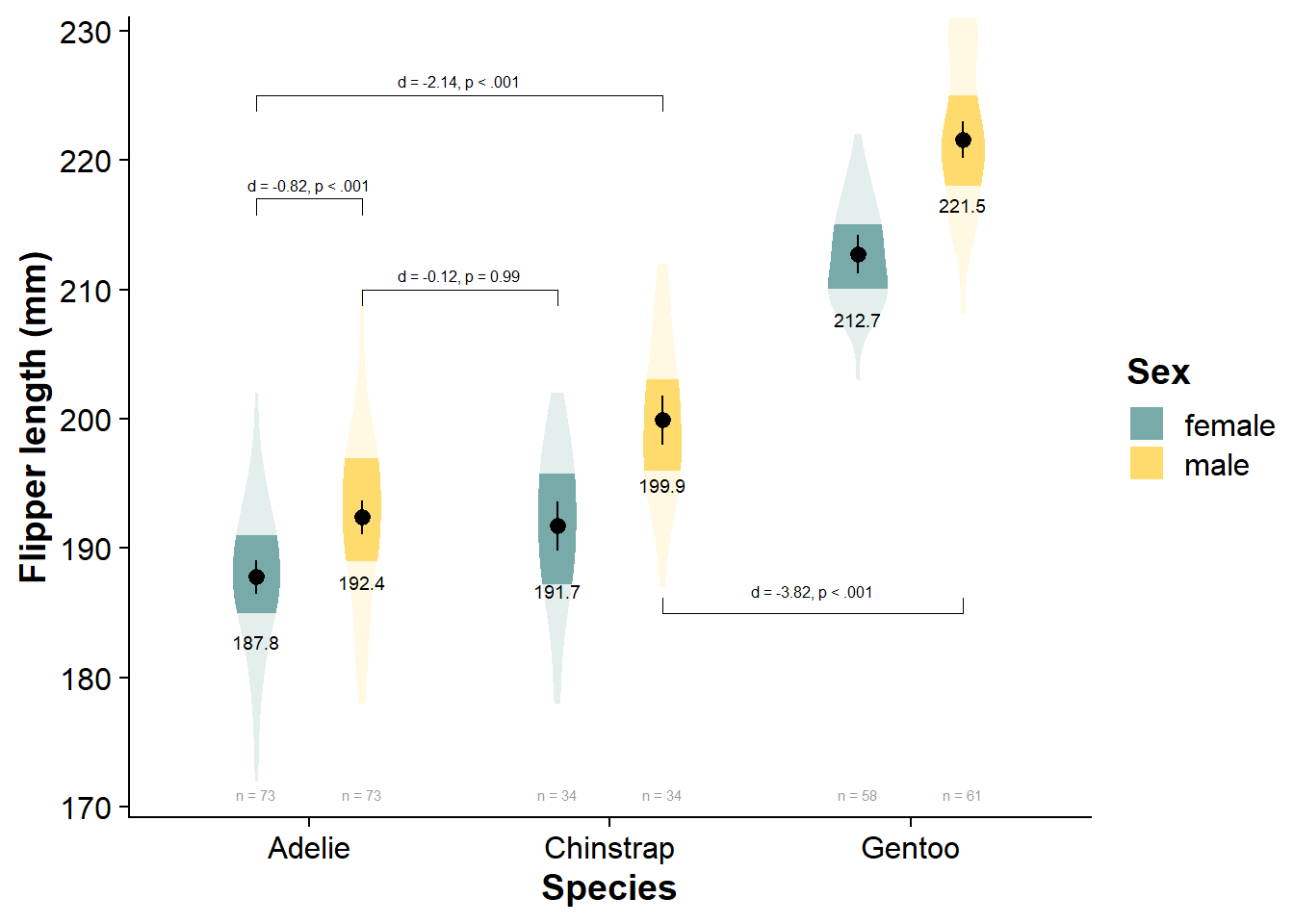
viofade_fact_bracket <- viofade_fact +
  ggpubr::geom_bracket(inherit.aes = FALSE, # necessary for factorial design
                       tip.length = 0.02,
                       vjust = 0,
                       xmin = 1.175, # You need to play with these by hand
                       xmax = 1.825,
                       y.position = 210 ,
                       label.size = 2.1,
                       label = paste0(
                         report_tidy_t(
                           flipper_fact_emmeans_contrasts[flipper_fact_emmeans_contrasts$contrast =="Chinstrap female - Adelie male",],
                           italicize = FALSE,
                           ci = FALSE)) # content of your bracket text


  ) +
  ggpubr::geom_bracket(inherit.aes = FALSE,
                       tip.length = 0.02,
                       vjust = 0,
                       xmin = .825,
                       xmax = 1.175,
                       y.position = 217 ,
                       label.size = 2.1,
                       label = paste0(
                         report_tidy_t(
                           flipper_fact_emmeans_contrasts[flipper_fact_emmeans_contrasts$contrast =="Adelie female - Adelie male",],
                           italicize = FALSE,
                           ci = FALSE)) # content of your bracket text
  ) +
  ggpubr::geom_bracket(inherit.aes = FALSE,
                       tip.length = 0.02,
                       vjust = 0,
                       xmin = .825,
                       xmax = 2.175,
                       y.position = 225 ,
                       label.size = 2.1,

                       label = paste0(
                         report_tidy_t(
                           flipper_fact_emmeans_contrasts[flipper_fact_emmeans_contrasts$contrast =="Adelie female - Chinstrap male",],
                           italicize = FALSE,
                           ci = FALSE)) # content of your bracket text
  ) +
  ggpubr::geom_bracket(inherit.aes = FALSE,
                       tip.length = -0.02,
                       vjust = 0.6,
                       xmin = 2.175,
                       xmax = 3.175,
                       y.position = 185 ,
                       label.size = 2.1,
                       label = paste0(
                         report_tidy_t(
                           flipper_fact_emmeans_contrasts[flipper_fact_emmeans_contrasts$contrast =="Chinstrap male - Gentoo male",],
                           italicize = FALSE,
                           ci = FALSE)) # content of your bracket text
  )


viofade_fact_bracket
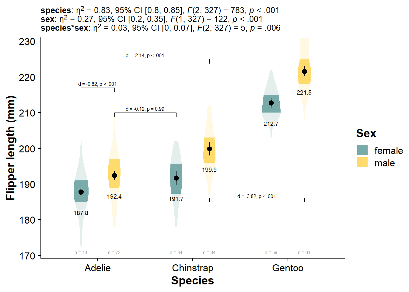
Click here if you want an ultra-stat-detailed plot
Not exactly the amount of information I would put in the graph, but you can really get your analysis fully integrated with the plot, just by using the same subtitle function as before:
 viofade_fact_bracket +
    labs(subtitle = paste0("**species**: ", report_tidy_anova_etaci(flipper_fact_anova,"species"), "<br>",
                           "**sex**: ", report_tidy_anova_etaci(flipper_fact_anova,"sex"), "<br>",
                           "**species*sex**: ",report_tidy_anova_etaci(flipper_fact_anova,"species:sex"))
         )  +
  theme(plot.subtitle = ggtext::element_markdown(size = 10))
Hopefully by the time you are reading this question will be answered
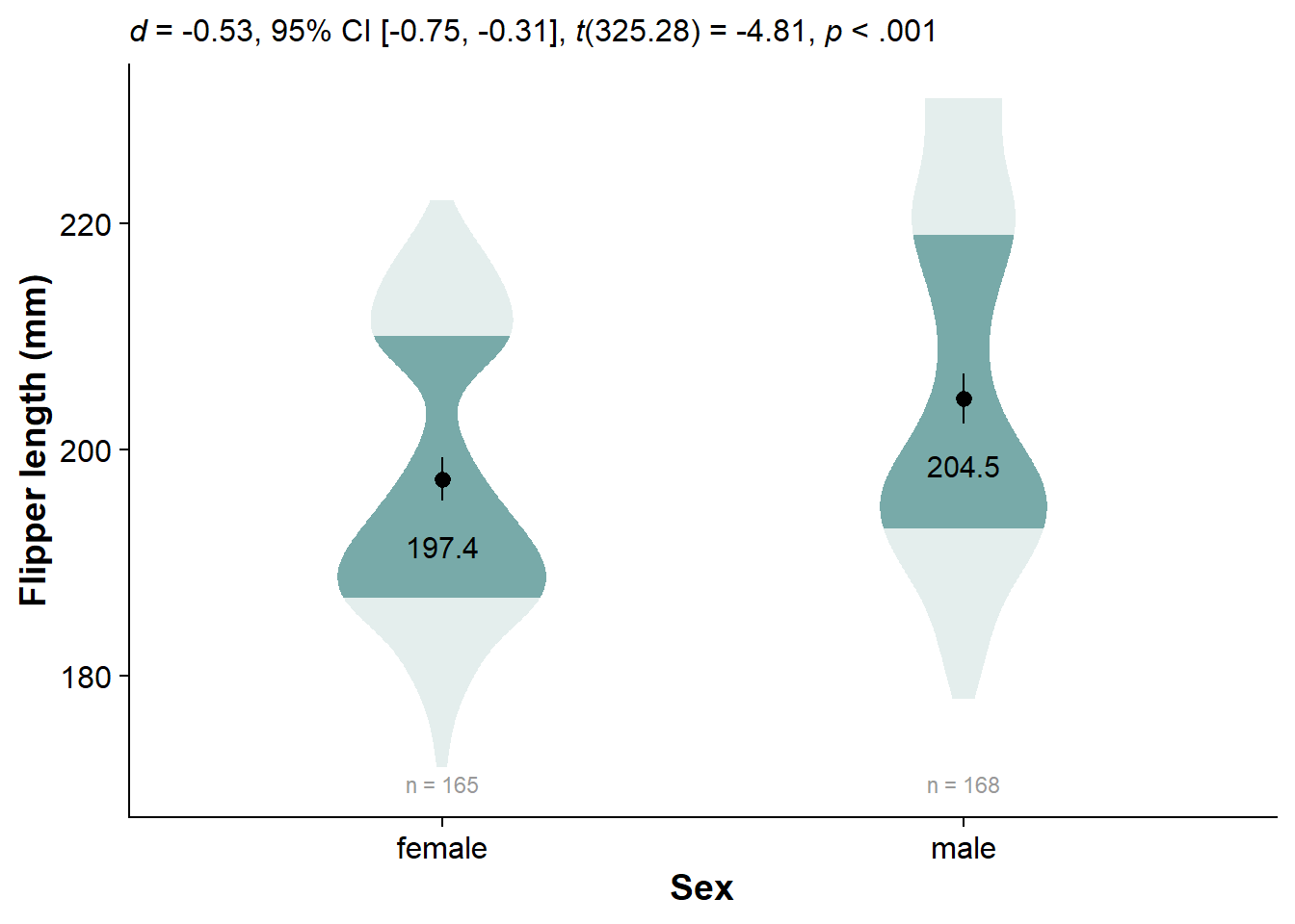
Now Compare Just Two Groups
Use our workhorse make_summary():
flipper_sex_summary <- make_summary(data = df, dv = flipper, grouping1 = sex)

knitr::kable(flipper_sex_summary)
| sex | mean | min | max | n | std_dev | se | y25 | y50 | y75 | loci | upci |
|---|---|---|---|---|---|---|---|---|---|---|---|
| female | 197.36 | 172 | 222 | 165 | 12.50 | 0.97 | 187 | 193 | 210 | 195.4988 | 199.3012 |
| male | 204.51 | 178 | 231 | 168 | 14.55 | 1.12 | 193 | 200 | 219 | 202.3048 | 206.6952 |
Run t a between-subjects t-test with t.test(), extract and format it with report::report() and data.frame(), and clean the names with janitor::clean_names():
flipper_sex_ttest <- t.test(flipper ~ sex, data=df) %>%
  report::report() %>%
  data.frame() %>%
  janitor::clean_names()

knitr::kable(flipper_sex_ttest)
| parameter | group | mean_group1 | mean_group2 | difference | ci | ci_low | ci_high | t | df_error | p | method | alternative | d | d_ci_low | d_ci_high |
|---|---|---|---|---|---|---|---|---|---|---|---|---|---|---|---|
| flipper | sex | 197.3636 | 204.506 | -7.142316 | 0.95 | -10.06481 | -4.219821 | -4.807866 | 325.2784 | 2.3e-06 | Welch Two Sample t-test | two.sided | -0.5331566 | -0.7539304 | -0.3115901 |
Now we can specify the whole plot, using everything we’ve learned:
ggplot(data = df, # specify the dataframe that we want to pull variables from
       aes(y = flipper, # our dependent/response/outcome variable
           x = sex  # our grouping/independent/predictor variable
       )) +
  # insert faded violin slab
  ggdist::stat_slab(side = "both",  # turn from slab to violin
                    aes(fill_ramp = stat(level)),  # specify shading
                    fill = nova_palette[1], # specify used to fill violin
                    .width = c(.50, 1), # specify shading quantiles
                    scale = .4) + # change size of violin
  # insert mean text
  geom_text(data = flipper_sex_summary, # our externally-defined summary dataframe
            aes(x = sex, # x-position of geom_text
                y = mean, # y-position of geom_text
                label = round(mean,1)), # actual content
            color="black",
            size = 4, # size of text
            vjust = 3.5) + # some vertical nudging downwards
  # Insert mean and 95% confidence interval
  geom_pointrange(data = flipper_sex_summary, # our externally-defined summary dataframe
                  aes(x = sex,  # our independent variable
                      y = mean, # our outcome/dependent variable
                      ymin = loci,  # lower-bound confidence interval
                      ymax = upci # upper-bound confidence interval
                  )) +
  # insert sample sizes
  geom_text(data = flipper_sex_summary, # specify our custom dataframe
            aes(label = paste("n =", n), # the actual text content
                y = flipper_summary[which.min(flipper_summary$min),]$mean -
                  3*flipper_summary[which.min(flipper_summary$min),]$std_dev), #  dynamically set the location of sample size (3 standard deviations below the mean of the lowest-scoring group)
            size = 3,  # size of text
            color = "grey60") +
  guides(fill_ramp = "none") + # get rid of legend element for fading quantiles
  cowplot::theme_half_open() + # nice theme for publication
  labs(subtitle = report_tidy_t(flipper_sex_ttest, test.stat = T)) + # test statistic
  theme(plot.subtitle = ggtext::element_markdown()) + # enable markdown styling
  theme(axis.title = element_text(face="bold")) + #bold axis titles
  ylab("Flipper length (mm)") + # change y-axis label
  xlab("Sex") # change x-axis label
Conclusion
One of the major strengths of R is also one of its most daunting aspects for newcomers: there are lots of ways to analyze and visualize your data. The aim of this post is to guide readers (my future self included) through a single, seamless workflow to bring data products together in a way that you can readily publish in reports, journal articles, theses, posters, presentations, and anything else. See my post on faded dotplots and shadeplots to see a variety of plotting alternatives.
Thanks for reading. I know we all have things to do and places to be.
Loaded Packages
Aphalo P (2023). ggpp: Grammar Extensions to ‘ggplot2’. R package version 0.5.2, <URL: https://CRAN.R-project.org/package=ggpp>.
Bates D, Mächler M, Bolker B, Walker S (2015). “Fitting Linear Mixed-Effects Models Using lme4.” Journal of Statistical Software, 67(1), 1-48. doi: 10.18637/jss.v067.i01 (URL: https://doi.org/10.18637/jss.v067.i01).
Bates D, Maechler M, Jagan M (2023). Matrix: Sparse and Dense Matrix Classes and Methods. R package version 1.5-4, <URL: https://CRAN.R-project.org/package=Matrix>.
Ben-Shachar MS, Lüdecke D, Makowski D (2020). “effectsize: Estimation of Effect Size Indices and Standardized Parameters.” Journal of Open Source Software, 5(56), 2815. doi: 10.21105/joss.02815 (URL: https://doi.org/10.21105/joss.02815), <URL: https://doi.org/10.21105/joss.02815>.
Firke S (2023). janitor: Simple Tools for Examining and Cleaning Dirty Data. R package version 2.2.0, <URL: https://CRAN.R-project.org/package=janitor>.
Fox J, Weisberg S (2019). An R Companion to Applied Regression, Third edition. Sage, Thousand Oaks CA. <URL: https://socialsciences.mcmaster.ca/jfox/Books/Companion/>.
Fox J, Weisberg S, Price B (2022). carData: Companion to Applied Regression Data Sets. R package version 3.0-5, <URL: https://CRAN.R-project.org/package=carData>.
Grolemund G, Wickham H (2011). “Dates and Times Made Easy with lubridate.” Journal of Statistical Software, 40(3), 1-25. <URL: https://www.jstatsoft.org/v40/i03/>.
Harrell Jr F (2023). Hmisc: Harrell Miscellaneous. R package version 5.1-0, <URL: https://CRAN.R-project.org/package=Hmisc>.
Horst AM, Hill AP, Gorman KB (2020). palmerpenguins: Palmer Archipelago (Antarctica) penguin data. doi: 10.5281/zenodo.3960218 (URL: https://doi.org/10.5281/zenodo.3960218), R package version 0.1.0, <URL: https://allisonhorst.github.io/palmerpenguins/>.
Kassambara A (2023). ggpubr: ‘ggplot2’ Based Publication Ready Plots. R package version 0.6.0, <URL: https://CRAN.R-project.org/package=ggpubr>.
Kay M (2023). ggdist: Visualizations of Distributions and Uncertainty. doi: 10.5281/zenodo.3879620 (URL: https://doi.org/10.5281/zenodo.3879620), R package version 3.3.0, <URL: https://mjskay.github.io/ggdist/>.
Lenth R (2023). emmeans: Estimated Marginal Means, aka Least-Squares Means. R package version 1.8.9, <URL: https://CRAN.R-project.org/package=emmeans>.
Makowski D, Lüdecke D, Patil I, Thériault R, Ben-Shachar M, Wiernik B (2023). “Automated Results Reporting as a Practical Tool to Improve Reproducibility and Methodological Best Practices Adoption.” CRAN. <URL: https://easystats.github.io/report/>.
Millard SP (2013). EnvStats: An R Package for Environmental Statistics. Springer, New York. ISBN 978-1-4614-8455-4, <URL: https://www.springer.com>.
Müller K, Wickham H (2023). tibble: Simple Data Frames. R package version 3.2.1, <URL: https://CRAN.R-project.org/package=tibble>.
Pasek J, Tahk wsafA, Culter scmfRAcbG, Schwemmle. M (2021). weights: Weighting and Weighted Statistics. R package version 1.0.4, <URL: https://CRAN.R-project.org/package=weights>.
R Core Team (2021). R: A Language and Environment for Statistical Computing. R Foundation for Statistical Computing, Vienna, Austria. <URL: https://www.R-project.org/>.
Singmann H, Bolker B, Westfall J, Aust F, Ben-Shachar M (2023). afex: Analysis of Factorial Experiments. R package version 1.3-0, <URL: https://CRAN.R-project.org/package=afex>.
Wickham H (2016). ggplot2: Elegant Graphics for Data Analysis. Springer-Verlag New York. ISBN 978-3-319-24277-4, <URL: https://ggplot2.tidyverse.org>.
Wickham H (2022). stringr: Simple, Consistent Wrappers for Common String Operations. R package version 1.5.0, <URL: https://CRAN.R-project.org/package=stringr>.
Wickham H (2023). forcats: Tools for Working with Categorical Variables (Factors). R package version 1.0.0, <URL: https://CRAN.R-project.org/package=forcats>.
Wickham H, Averick M, Bryan J, Chang W, McGowan LD, François R, Grolemund G, Hayes A, Henry L, Hester J, Kuhn M, Pedersen TL, Miller E, Bache SM, Müller K, Ooms J, Robinson D, Seidel DP, Spinu V, Takahashi K, Vaughan D, Wilke C, Woo K, Yutani H (2019). “Welcome to the tidyverse.” Journal of Open Source Software, 4(43), 1686. doi: 10.21105/joss.01686 (URL: https://doi.org/10.21105/joss.01686).
Wickham H, François R, Henry L, Müller K, Vaughan D (2023). dplyr: A Grammar of Data Manipulation. R package version 1.1.2, <URL: https://CRAN.R-project.org/package=dplyr>.
Wickham H, Henry L (2023). purrr: Functional Programming Tools. R package version 1.0.1, <URL: https://CRAN.R-project.org/package=purrr>.
Wickham H, Hester J, Bryan J (2023). readr: Read Rectangular Text Data. R package version 2.1.4, <URL: https://CRAN.R-project.org/package=readr>.
Wickham H, Vaughan D, Girlich M (2023). tidyr: Tidy Messy Data. R package version 1.3.0, <URL: https://CRAN.R-project.org/package=tidyr>.
Wilke C (2020). cowplot: Streamlined Plot Theme and Plot Annotations for ‘ggplot2’. R package version 1.1.1, <URL: https://CRAN.R-project.org/package=cowplot>.
Wilke C, Wiernik B (2022). ggtext: Improved Text Rendering Support for ‘ggplot2’. R package version 0.1.2, <URL: https://CRAN.R-project.org/package=ggtext>.

Code Dump
Click here to see absolutely all the code in this post:
# Load-packages ------------------------------------------------------------------
library(palmerpenguins) # dataset
library(cowplot) # publication-ready plots
library(tidyverse) # ggplot and tidy functions
library(ggdist) # density slabs
library(EnvStats) # stat_n_text() for inserting sample sizes
library(ggtext) # formatting text elements with markdown syntax
library(afex) # anova functions
library(car) # anova functions
library(emmeans) # estimated marginal means and pairwise comparisons
library(effectsize) # effect sizes
library(ggpubr) # significance brackets
library(weights) # rounding values
library(report) # for citing packages
library(janitor) #for cleaning variable names
library(ggpp) # for position_dodge2nudge
# Define color palette
nova_palette <- c("#78AAA9", "#FFDB6E")
# define functions -----------------------------------------------------------
# This function generates a summary table with various statistics for the specified grouping variables and dependent variable.
make_summary <- function(data, dv, grouping1, grouping2, grouping3){
# Use dplyr to group the data by the specified grouping variables and calculate summary statistics
data %>%
group_by({{grouping1}}, {{grouping2}}, {{grouping3}}) %>% # Group by the specified variables
dplyr::summarise(
mean = round(mean({{dv}}), 2), # Calculate and round the mean of the dependent variable
min = round(min({{dv}}), 2), # Calculate and round the minimum
max = round(max({{dv}}), 2), # Calculate and round the maximum
n = n(), # Count the number of observations
std_dev = round(sd({{dv}}), 2), # Calculate and round the standard deviation
se = round(sd({{dv}}) / sqrt(n()), 2), # Calculate and round the standard error
y25 = round(quantile({{dv}}, 0.25)), # Calculate and round the 25th percentile
y50 = round(median({{dv}})), # Calculate and round the median (50th percentile)
y75 = round(quantile({{dv}}, 0.75)), # Calculate and round the 75th percentile
loci = round(mean({{dv}}), 1) - 1.96 * se, # Calculate and round the lower confidence interval
upci = round(mean({{dv}}), 1) + 1.96 * se # Calculate and round the upper confidence interval
)
}
#We can make a custom function calculate_and_merge_effect_sizes() to loop compute cohen’s d for each comparison, then merge the effect sizes in our flipper_emmeans_contrasts dataframe:
calculate_and_merge_effect_sizes <- function(emmeans, model) {
contrasts <- data.frame(emmeans$contrasts)
emmean_d <- data.frame(emmeans::eff_size(
emmeans,
method = "pairwise",
sigma = sigma(model),
edf = df.residual(model)))
combined_dataframe <- data.frame(contrasts, emmean_d)
# Rename some columns for clarity
combined_dataframe <- combined_dataframe %>%
select(-contrast.1, -df.1)%>%
rename(d = effect.size,
d_ci_low = lower.CL,
d_ci_high = upper.CL,
d_se = SE.1,
df_error = df,
p = p.value)
# Return the combined dataframe with effect size results
return(combined_dataframe)
}
# Make a custom function, merge_emmeans_summary(), to merge summary and emmeans. Particularly useful for multivariate analyses:
#merging regular summary stats with emmeans
# This function takes summary data and a tidy emmeans object and adds emmeans-related columns to the summary data
merge_emmeans_summary <- function(summary_data, emmeans_tidy) {
# Add emmeans-related columns to the summary_data
# Assign the 'emmean' values from the emmeans_tidy to a new column 'emmean' in summary_data
summary_data$emmean <- emmeans_tidy$emmean
# Assign the 'SE' values from emmeans_tidy to a new column 'emmean_se' in summary_data
summary_data$emmean_se <- emmeans_tidy$SE
# Assign the 'lower.CL' values from emmeans_tidy to a new column 'emmean_loci' in summary_data
summary_data$emmean_loci <- emmeans_tidy$lower.CL
# Assign the 'upper.CL' values from emmeans_tidy to a new column 'emmean_upci' in summary_data
summary_data$emmean_upci <- emmeans_tidy$upper.CL
# Return the summary_data with the added emmeans-related columns
return(summary_data)
}
# This function generates a text summary based on user-specified options using a tidy t-test dataframe.
report_tidy_t <- function(tidy_frame,
italicize = TRUE,
ci = TRUE,
ci.lab = TRUE,
test.stat = FALSE,
point = TRUE,
pval = TRUE,
pval_comma = TRUE
){
# Initialize an empty string to store the result text
text <- ""
# Conditionally add effect size (d) to the result text
if (point == TRUE) {
text <- paste0(text,
ifelse(italicize == TRUE, "*d* = ", "d = "), # Italicized or not
round(tidy_frame$d, 2) # Rounded d value
)
}
# Conditionally add 95% CI to the result text
if (ci == TRUE) {
text <- paste0(text,
ifelse(ci.lab == TRUE,
paste0(", 95% CI [",
round(tidy_frame$d_ci_low, 2), ", ",
round(tidy_frame$d_ci_high, 2), "]"), # Label and rounded CI values
paste0(" [",
round(tidy_frame$d_ci_low, 2), ", ",
round(tidy_frame$d_ci_high, 2), "]") # Only rounded CI values
)
)
}
# Conditionally add t-statistic and degrees of freedom to the result text
if (test.stat == TRUE) {
text <- paste0(text,
", *t*(", round(tidy_frame$df_error, 2), ") = ", round(tidy_frame$t, 2) # t-statistic and df
)
}
# Conditionally add p-value to the result text
if (pval == TRUE) {
text <- paste0(text,
ifelse(pval_comma == TRUE,
ifelse(italicize == TRUE, ", *p* ", ", p "),
ifelse(italicize == TRUE, "*p* ", "p ") # Italicized or not
),
ifelse(tidy_frame$p < .001, "< .001", # Formatting based on p-value
ifelse(tidy_frame$p > .01,
paste("=", tidy_frame$p %>% round(2)),
paste("=", tidy_frame$p %>% round(3))
)
)
)
}
# Return the generated text summary
return(text)
}
# This function formats a p-value and optionally italicizes it for reporting.
report_pval_full <- function(pval, italicize = TRUE) {
# Check if the p-value is less than .001
if (pval < .001) {
# If p-value is very small, format it as "*p* < .001" (with or without italics)
result <- ifelse(italicize == TRUE, "*p* < .001", "p < .001")
} else {
# If p-value is not very small, format it as "*p* = " with either 2 or 3 decimal places
if (pval >= .01) {
# Use 2 decimal places for p-values >= .01
result <- ifelse(italicize == TRUE, "*p*", "p") # Start with "*p*" or "p"
result <- paste0(result, " = ", weights::rd(pval, 2)) # Append the formatted p-value
} else {
# Use 3 decimal places for p-values less than .01
result <- ifelse(italicize == TRUE, "*p*", "p") # Start with "*p*" or "p"
result <- paste0(result, " = ", weights::rd(pval, 3)) # Append the formatted p-value
}
}
# Return the formatted p-value
return(result)
}
# This function generates a text summary of ANOVA results based on user-specified options.
report_tidy_anova_etaci <- function(tidy_frame, # Your tidy ANOVA dataframe
term, # The predictor in your tidy ANOVA dataframe
effsize = TRUE, # Display the effect size
ci95 = TRUE, # Display the 95% CI
ci.lab = TRUE, # Display the "95% CI" label
teststat = TRUE, # Display the F-score and degrees of freedom
pval = TRUE # Display the p-value
){
# Initialize an empty string to store the result text
text <- ""
# Conditionally add effect size (eta square) to the result text
if (effsize == TRUE) {
text <- paste0(text,
"\u03b7^2^ = ", # Unicode for eta square
round(as.numeric(tidy_frame[term, "pes"]), 2)
)
}
# Conditionally add 95% CI to the result text
if (ci95 == TRUE) {
text <- paste0(text,
ifelse(ci.lab == TRUE,
paste0(", 95% CI ["), " ["),
round(as.numeric(tidy_frame[term, "pes_ci95_lo"]), 2), ", ",
round(as.numeric(tidy_frame[term, "pes_ci95_hi"]), 2), "]"
)
}
# Conditionally add F-score and degrees of freedom to the result text
if (teststat == TRUE) {
text <- paste0(text,
", *F*(", tidy_frame[term, "Df"],
", ", tidy_frame["Residuals", "Df"], ") = ",
round(as.numeric(tidy_frame[term, "F.value"], 2))
)
}
# Conditionally add p-value to the result text
if (pval == TRUE) {
text <- paste0(text,
", ", report_pval_full(tidy_frame[term, "Pr..F."])
)
}
# Return the generated text summary
return(text)
}
# load-data ------------------------------------------------------------------
# assigns data to a dataframe we call "df"
df <- palmerpenguins::penguins
# drop rows with missing values
df <- df[complete.cases(df)==TRUE, ]
df <- rename(df, flipper = flipper_length_mm)
# peek at the structure of our dataframe
str(df)
# create summary dataframe --------------------------------------------
# Apply our custom function to create summary dataframe
flipper_summary <- make_summary(data = df, dv = flipper, grouping1 = species)
# Show summary dataframe in table
knitr::kable(flipper_summary)
# analysis ------------------------------------------------------------------
# Anova with stats::aov() and car::Anova():
# Fit data
flipper_fit <- stats::aov(flipper ~ species, data = df)
# Run anova
flipper_anova <- car::Anova(flipper_fit)
#Calculate effect sizes with effectsize::eta_squared(), and import them into the ANOVA table:
# Extract effect size (partial eta squared) from anova
flipper_anova_pes <- effectsize::eta_squared(flipper_anova,
alternative="two.sided",
verbose = FALSE)
# Convert anova table into dataframe
flipper_anova <- data.frame(flipper_anova)
# import effect size estimates and confidence intervals to anova dataframe
flipper_anova$pes_ci95_lo <- flipper_anova_pes$CI_low
flipper_anova$pes_ci95_hi <- flipper_anova_pes$CI_high
flipper_anova$pes <- flipper_anova_pes$Eta2
# round all numeric columns to 2 decimal places
flipper_anova <- flipper_anova %>%
dplyr::mutate_if(is.numeric, function(x) round(x, 2))
# display anova dataframe
knitr::kable(flipper_anova)
# Estimated marginal means --------------------------
# Extract estimated marginal means
flipper_emmeans <- emmeans::emmeans(flipper_fit, specs = pairwise ~ species)
# convert estimated marginal mean contrasts to dataframe
flipper_emmeans_contrasts <- data.frame(flipper_emmeans$contrasts)
# Convert estimated marginal means to dataframe
flipper_emmeans_tidy <- data.frame(flipper_emmeans$emmeans)
# Use merge_emmeans_summary() to combine with our basic flipper_summary into a single model-enhanced dataframe:
# Order the dataframes based on dependent variables - Not necessary here, but good practice that helps for factorial designs
flipper_summary <- flipper_summary[order(flipper_summary$species), ]
flipper_emmeans_tidy <- flipper_emmeans_tidy[order(flipper_emmeans_tidy$species), ]
# merge dataframes
flipper_summary <- merge_emmeans_summary(summary_data = flipper_summary,
emmeans_tidy = flipper_emmeans_tidy)
# Round numeric values
flipper_summary <- flipper_summary %>%
mutate_if(is.numeric, function(x) round(x, 2))
flipper_summary
#merge estimated marginal mean contrasts with their effect sizes:
flipper_emmeans_contrasts <- calculate_and_merge_effect_sizes(flipper_emmeans, flipper_fit)
flipper_emmeans_contrasts
# visualize data -------------------
ggplot(data = df, # specify the dataframe that we want to pull variables from
aes(y = flipper, # our dependent/response/outcome variable
x = species # our grouping/independent/predictor variable
)) +
cowplot::theme_half_open() + # nice theme for publication
ggdist::stat_slab(side = "both", # turn from slab to violin
aes(fill_ramp = stat(level)), # specify shading
fill = nova_palette[1], # specify used to fill violin
.width = c(.50, 1), # specify shading quantiles
scale = .4) + # change size of violin
geom_pointrange(data = flipper_summary, # our externally-defined summary dataframe
aes(x = species, # our independent variable
y = mean, # our outcome/dependent variable
ymin = loci, # lower-bound confidence interval
ymax = upci # upper-bound confidence interval
)) +
geom_text(data = flipper_summary, aes(x = species,
y = mean,
label = round(mean,1)),
color="black",
size = 2.5,
vjust = 5) +
geom_text(data = flipper_summary,
aes(label = paste("n =", n),
y = flipper_summary[which.min(flipper_summary$min),]$mean -
3*flipper_summary[which.min(flipper_summary$min),]$std_dev), # dynamically set the location of sample size (3 standard deviations below the mean of the lowest-scoring group)
size = 2,
color = "grey60") +
guides(fill_ramp = "none") + # get rid of legend element for fading quantiles
labs(subtitle = report_tidy_anova_etaci(flipper_anova,"species")) +
theme(plot.subtitle = ggtext::element_markdown()) +
ggpubr::geom_bracket(
tip.length = 0.02, # the downard "tips" of the bracket
vjust = 0, # moves your text label (in this case, the p-value)
xmin = 1, #starting point for the bracket
xmax = 2, # ending point for the bracket
y.position = 220, # vertical location of the bracket
label.size = 2.5, # size of your bracket text
label = paste0(
report_tidy_t(
flipper_emmeans_contrasts[flipper_emmeans_contrasts$contrast =="Adelie - Chinstrap",],
italicize = FALSE,
ci = FALSE)) # content of your bracket text
) +
ggpubr::geom_bracket(
tip.length = 0.02,
vjust = 0,
xmin = 2,
xmax = 3,
y.position = 227 ,
label.size = 2.5,
label = paste0("My hypothesis, ",
report_tidy_t(flipper_emmeans_contrasts[flipper_emmeans_contrasts$contrast =="Chinstrap - Gentoo",],
italicize = FALSE,
ci = FALSE,
point = FALSE,
pval_comma= FALSE))
# label = paste0("My hypothesis, ",
# report_pval_full(flipper_emmeans_contrasts[flipper_emmeans_contrasts$contrast ==
# 'Chinstrap - Gentoo', "p"], italicize = FALSE))
#
)+
theme(axis.title = element_text(face="bold")) +
ylab("Flipper length (mm)") +
xlab("Species")
ggsave(here::here("figures", "viofade.png"),
width=7, height = 3, dpi=700)
library(palmerpenguins) # dataset
library(cowplot) # publication-ready plots
library(tidyverse) # ggplot and tidy functions
library(ggdist) # density slabs
library(EnvStats) # stat_n_text() for inserting sample sizes
library(ggtext) # formatting text elements with markdown syntax
library(afex) # anova functions
library(car) # anova functions
library(emmeans) # estimated marginal means and pairwise comparisons
library(effectsize) # effect sizes
library(ggpubr) # significance brackets
library(weights) # rounding values
library(report) # for citing packages
library(janitor) #for cleaning variable names
library(ggpp) # for position_dodge2nudge
# Define color palette
nova_palette <- c("#78AAA9", "#FFDB6E")
# assigns data to a dataframe we call "df"
df <- palmerpenguins::penguins
# drop rows with missing values
df <- df[complete.cases(df)==TRUE, ]
df <- rename(df, flipper = flipper_length_mm)
# peek at the structure of our dataframe
str(df)
# This function generates a summary table with various statistics for the specified grouping variables and dependent variable.
make_summary <- function(data, dv, grouping1, grouping2, grouping3){
# Use dplyr to group the data by the specified grouping variables and calculate summary statistics
data %>%
group_by({{grouping1}}, {{grouping2}}, {{grouping3}}) %>% # Group by the specified variables
dplyr::summarise(
mean = round(mean({{dv}}), 2), # Calculate and round the mean of the dependent variable
min = round(min({{dv}}), 2), # Calculate and round the minimum
max = round(max({{dv}}), 2), # Calculate and round the maximum
n = n(), # Count the number of observations
std_dev = round(sd({{dv}}), 2), # Calculate and round the standard deviation
se = round(sd({{dv}}) / sqrt(n()), 2), # Calculate and round the standard error
y25 = round(quantile({{dv}}, 0.25)), # Calculate and round the 25th percentile
y50 = round(median({{dv}})), # Calculate and round the median (50th percentile)
y75 = round(quantile({{dv}}, 0.75)), # Calculate and round the 75th percentile
loci = round(mean({{dv}}), 1) - 1.96 * se, # Calculate and round the lower confidence interval
upci = round(mean({{dv}}), 1) + 1.96 * se # Calculate and round the upper confidence interval
)
}
# Apply our custom function to create summary dataframe
flipper_summary <- make_summary(data = df, dv = flipper, grouping1 = species)
# Show summary dataframe in table
knitr::kable(flipper_summary)
# Setting contrasts
contrasts(df$species) <- contr.sum
contrasts(df$sex) <- contr.sum
# Fit data
flipper_fit <- stats::aov(flipper ~ species, data = df)
# Run anova
flipper_anova <- car::Anova(flipper_fit)
# Extract effect size (partial eta squared) from anova
flipper_anova_pes <- effectsize::eta_squared(flipper_anova,
alternative="two.sided",
verbose = FALSE)
# Convert anova table into dataframe
flipper_anova <- data.frame(flipper_anova)
# import effect size estimates and confidence intervals to anova dataframe
flipper_anova$pes_ci95_lo <- flipper_anova_pes$CI_low
flipper_anova$pes_ci95_hi <- flipper_anova_pes$CI_high
flipper_anova$pes <- flipper_anova_pes$Eta2
# round all numeric columns to 2 decimal places
flipper_anova <- flipper_anova %>%
dplyr::mutate_if(is.numeric, function(x) round(x, 2))
# display anova dataframe
knitr::kable(flipper_anova)
# Extract estimated marginal means
flipper_emmeans <- emmeans::emmeans(flipper_fit, specs = pairwise ~ species)
# Convert estimated marginal means to dataframe
flipper_emmeans_tidy <- data.frame(flipper_emmeans$emmeans)
# This function takes summary data and a tidy emmeans object and adds emmeans-related columns to the summary data
merge_emmeans_summary <- function(summary_data, emmeans_tidy) {
# Add emmeans-related columns to the summary_data
# Assign the 'emmean' values from the emmeans_tidy to a new column 'emmean' in summary_data
summary_data$emmean <- emmeans_tidy$emmean
# Assign the 'SE' values from emmeans_tidy to a new column 'emmean_se' in summary_data
summary_data$emmean_se <- emmeans_tidy$SE
# Assign the 'lower.CL' values from emmeans_tidy to a new column 'emmean_loci' in summary_data
summary_data$emmean_loci <- emmeans_tidy$lower.CL
# Assign the 'upper.CL' values from emmeans_tidy to a new column 'emmean_upci' in summary_data
summary_data$emmean_upci <- emmeans_tidy$upper.CL
# Return the summary_data with the added emmeans-related columns
return(summary_data)
}
# Order the dataframes based on dependent variables - Not necessary here, but good practice that helps for factorial designs
flipper_summary <- flipper_summary[order(flipper_summary$species), ]
flipper_emmeans_tidy <- flipper_emmeans_tidy[order(flipper_emmeans_tidy$species), ]
# merge dataframes
flipper_summary <- merge_emmeans_summary(summary_data = flipper_summary,
emmeans_tidy = flipper_emmeans_tidy)
# Round numeric values
flipper_summary <- flipper_summary %>%
mutate_if(is.numeric, function(x) round(x, 2))
knitr::kable(flipper_summary)
# convert estimated marginal mean contrasts to dataframe
flipper_emmeans_contrasts <- data.frame(flipper_emmeans$contrasts)
# This function takes a dataframe, a column name for t-values, a column name for degrees of freedom, and a prefix for result column names.
calculate_and_merge_effect_sizes <- function(emmeans, model) {
contrasts <- data.frame(emmeans$contrasts)
emmean_d <- data.frame(emmeans::eff_size(
emmeans,
method = "pairwise",
sigma = sigma(model),
edf = df.residual(model)))
combined_dataframe <- data.frame(contrasts, emmean_d)
# Rename some columns for clarity
combined_dataframe <- combined_dataframe %>%
select(-contrast.1, -df.1)%>%
rename(d = effect.size,
d_ci_low = lower.CL,
d_ci_high = upper.CL,
d_se = SE.1,
df_error = df,
p = p.value)
# Return the combined dataframe with effect size results
return(combined_dataframe)
}
flipper_emmeans_contrasts <- calculate_and_merge_effect_sizes(flipper_emmeans, flipper_fit)
knitr::kable(flipper_emmeans_contrasts)
# This function formats a p-value and optionally italicizes it for reporting.
report_pval_full <- function(pval, italicize = TRUE) {
# Check if the p-value is less than .001
if (pval < .001) {
# If p-value is very small, format it as "*p* < .001" (with or without italics)
result <- ifelse(italicize == TRUE, "*p* < .001", "p < .001")
} else {
# If p-value is not very small, format it as "*p* = " with either 2 or 3 decimal places
if (pval >= .01) {
# Use 2 decimal places for p-values >= .01
result <- ifelse(italicize == TRUE, "*p*", "p") # Start with "*p*" or "p"
result <- paste0(result, " = ", weights::rd(pval, 2)) # Append the formatted p-value
} else {
# Use 3 decimal places for p-values less than .01
result <- ifelse(italicize == TRUE, "*p*", "p") # Start with "*p*" or "p"
result <- paste0(result, " = ", weights::rd(pval, 3)) # Append the formatted p-value
}
}
# Return the formatted p-value
return(result)
}
flipper_emmeans_contrasts <- flipper_emmeans_contrasts %>%
mutate_if(is.numeric, function(x) round(x, 2))
knitr::kable(flipper_emmeans_contrasts)
# This function generates a text summary based on user-specified options using a tidy t-test dataframe.
report_tidy_t <- function(tidy_frame,
italicize = TRUE,
ci = TRUE,
ci.lab = TRUE,
test.stat = FALSE,
point = TRUE,
pval = TRUE,
pval_comma = TRUE
){
# Initialize an empty string to store the result text
text <- ""
# Conditionally add effect size (d) to the result text
if (point == TRUE) {
text <- paste0(text,
ifelse(italicize == TRUE, "*d* = ", "d = "), # Italicized or not
round(tidy_frame$d, 2) # Rounded d value
)
}
# Conditionally add 95% CI to the result text
if (ci == TRUE) {
text <- paste0(text,
ifelse(ci.lab == TRUE,
paste0(", 95% CI [",
round(tidy_frame$d_ci_low, 2), ", ",
round(tidy_frame$d_ci_high, 2), "]"), # Label and rounded CI values
paste0(" [",
round(tidy_frame$d_ci_low, 2), ", ",
round(tidy_frame$d_ci_high, 2), "]") # Only rounded CI values
)
)
}
# Conditionally add t-statistic and degrees of freedom to the result text
if (test.stat == TRUE) {
text <- paste0(text,
", *t*(", round(tidy_frame$df_error, 2), ") = ", round(tidy_frame$t, 2) # t-statistic and df
)
}
# Conditionally add p-value to the result text
if (pval == TRUE) {
text <- paste0(text,
ifelse(pval_comma == TRUE,
ifelse(italicize == TRUE, ", *p* ", ", p "),
ifelse(italicize == TRUE, "*p* ", "p ") # Italicized or not
),
ifelse(tidy_frame$p < .001, "< .001", # Formatting based on p-value
ifelse(tidy_frame$p > .01,
paste("=", tidy_frame$p %>% round(2)),
paste("=", tidy_frame$p %>% round(3))
)
)
)
}
# Return the generated text summary
return(text)
}
canvas <- ggplot(data = df, # specify the dataframe that we want to pull variables from
aes(y = flipper, # our dependent/response/outcome variable
x = species # our grouping/independent/predictor variable
))
canvas
canvas <- canvas +
cowplot::theme_half_open() # nice theme for publication
canvas # display our blank canvas
canvas + # this is our previously-defined canvas object, it passes the appropriate variables and theme
# This function puts out the dot-whisker for the mean + 95% CI
geom_pointrange(data = flipper_summary, # our externally-defined summary dataframe
aes(x = species, # our independent variable
y = mean, # our outcome/dependent variable
ymin = loci, # lower-bound confidence interval
ymax = upci # upper-bound confidence interval
))
canvas +
# density slab
ggdist::stat_slab() + # add a density slab
geom_pointrange(data = flipper_summary, # our externally-defined summary dataframe
aes(x = species, # our independent variable
y = mean, # our outcome/dependent variable
ymin = loci, # lower-bound confidence interval
ymax = upci # upper-bound confidence interval
))
canvas +
# density slab
ggdist::stat_slab(
side = "both") + # change the density slab to violin
geom_pointrange(data = flipper_summary, # our externally-defined summary dataframe
aes(x = species, # our independent variable
y = mean, # our outcome/dependent variable
ymin = loci, # lower-bound confidence interval
ymax = upci # upper-bound confidence interval
))
canvas +
# density slab
ggdist::stat_slab(side = "both",
fill = nova_palette[1]) + # color the violin geom with desired color
geom_pointrange(data = flipper_summary, # our externally-defined summary dataframe
aes(x = species, # our independent variable
y = mean, # our outcome/dependent variable
ymin = loci, # lower-bound confidence interval
ymax = upci # upper-bound confidence interval
))
canvas +
# density slab
ggdist::stat_slab(side = "both",
fill = nova_palette[1],
aes(fill_ramp = stat(level))) + # fade violins according to their quantile grouping
geom_pointrange(data = flipper_summary, # our externally-defined summary dataframe
aes(x = species, # our independent variable
y = mean, # our outcome/dependent variable
ymin = loci, # lower-bound confidence interval
ymax = upci # upper-bound confidence interval
))
canvas +
# density slab
ggdist::stat_slab(side = "both",
aes(fill_ramp = stat(level)),
fill = nova_palette[1],
.width = c(.50, 1)) + # change quantiles for shading from 66% to 50% (and eliminate the 95% shading)
geom_pointrange(data = flipper_summary, # our externally-defined summary dataframe
aes(x = species, # our independent variable
y = mean, # our outcome/dependent variable
ymin = loci, # lower-bound confidence interval
ymax = upci # upper-bound confidence interval
))
canvas +
# density slab
ggdist::stat_slab(side = "both",
aes(fill_ramp = stat(level)),
fill = nova_palette[1],
.width = c(.50, 1),
scale = .4) + # adjust slab width
geom_pointrange(data = flipper_summary, # our externally-defined summary dataframe
aes(x = species, # our independent variable
y = mean, # our outcome/dependent variable
ymin = loci, # lower-bound confidence interval
ymax = upci # upper-bound confidence interval
))
viofade <- canvas +
# density slab
ggdist::stat_slab(side = "both",
aes(fill_ramp = stat(level)),
fill = nova_palette[1],
.width = c(.50, 1),
scale = .4) +
geom_pointrange(data = flipper_summary, # our externally-defined summary dataframe
aes(x = species, # our independent variable
y = mean, # our outcome/dependent variable
ymin = loci, # lower-bound confidence interval
ymax = upci # upper-bound confidence interval
)) +
guides(fill_ramp = "none") # get rid of legend element for fading quantiles
viofade
viofade +
geom_text(data = flipper_summary,
aes(x = species,
y = mean,
label = round(mean,1)),
color="black",
size = 4,
vjust = 5)
# You could use this function if you want:
# stat_summary(aes(label = round(..y..,1)),
# fun = mean,
# geom = "text",vjust = 5)
viofade_text <- viofade +
geom_text(data = flipper_summary, aes(x = species,
y = mean,
label = round(mean,1)),
color="black",
size = 4,
vjust = 5) +
geom_text(data = flipper_summary,
aes(label = paste("n =", n),
y = flipper_summary[which.min(flipper_summary$min),]$mean -
3*flipper_summary[which.min(flipper_summary$min),]$std_dev), # dynamically set the location of sample size (3 standard deviations below the mean of the lowest-scoring group)
size = 3,
color = "grey60")
# You could use this for sample sizes if you want
# EnvStats::stat_n_text(color = "grey60")
viofade_text
# This function generates a text summary of ANOVA results based on user-specified options.
report_tidy_anova_etaci <- function(tidy_frame, # Your tidy ANOVA dataframe
term, # The predictor in your tidy ANOVA dataframe
effsize = TRUE, # Display the effect size
ci95 = TRUE, # Display the 95% CI
ci.lab = TRUE, # Display the "95% CI" label
teststat = TRUE, # Display the F-score and degrees of freedom
pval = TRUE # Display the p-value
){
# Initialize an empty string to store the result text
text <- ""
# Conditionally add effect size (eta square) to the result text
if (effsize == TRUE) {
text <- paste0(text,
"\u03b7^2^ = ", # Unicode for eta square
round(as.numeric(tidy_frame[term, "pes"]), 2)
)
}
# Conditionally add 95% CI to the result text
if (ci95 == TRUE) {
text <- paste0(text,
ifelse(ci.lab == TRUE,
paste0(", 95% CI ["), " ["),
round(as.numeric(tidy_frame[term, "pes_ci95_lo"]), 2), ", ",
round(as.numeric(tidy_frame[term, "pes_ci95_hi"]), 2), "]"
)
}
# Conditionally add F-score and degrees of freedom to the result text
if (teststat == TRUE) {
text <- paste0(text,
", *F*(", tidy_frame[term, "Df"],
", ", tidy_frame["Residuals", "Df"], ") = ",
round(as.numeric(tidy_frame[term, "F.value"], 2))
)
}
# Conditionally add p-value to the result text
if (pval == TRUE) {
text <- paste0(text,
", ", report_pval_full(tidy_frame[term, "Pr..F."])
)
}
# Return the generated text summary
return(text)
}
viofade_text +
labs(subtitle = report_tidy_anova_etaci(flipper_anova,"species"))
viofade_text_stats <- viofade_text +
labs(subtitle = report_tidy_anova_etaci(flipper_anova,"species")) +
theme(plot.subtitle = ggtext::element_markdown())
viofade_text_stats
viofade_text +
labs(subtitle = report_tidy_anova_etaci(flipper_anova,
"species",
teststat = FALSE,
pval = FALSE)) +
theme(plot.subtitle = ggtext::element_markdown())
viofade_text_stats_bracket1 <- viofade_text_stats +
ggpubr::geom_bracket(
tip.length = 0.02, # the downard "tips" of the bracket
vjust = 0, # moves your text label (in this case, the p-value)
xmin = 1, #starting point for the bracket
xmax = 2, # ending point for the bracket
y.position = 220, # vertical location of the bracket
label.size = 2.5, # size of your bracket text
label = paste0(
report_tidy_t(
flipper_emmeans_contrasts[flipper_emmeans_contrasts$contrast =="Adelie - Chinstrap",],
italicize = FALSE,
ci = FALSE)) # content of your bracket text
)
viofade_text_stats_bracket1
viofade_text_stats_bracket2 <- viofade_text_stats_bracket1 +
ggpubr::geom_bracket(
tip.length = 0.02,
vjust = 0,
xmin = 2,
xmax = 3,
y.position = 227 ,
label.size = 2.5,
label = paste0("My hypothesis, ",
report_tidy_t(flipper_emmeans_contrasts[flipper_emmeans_contrasts$contrast =="Adelie - Chinstrap",],
italicize = FALSE,
ci = FALSE,
point = FALSE,
pval_comma= FALSE))
)
viofade_text_stats_bracket2 +
theme(axis.title = element_text(face="bold")) +
ylab("Flipper length (mm)") +
xlab("Species")
dark_aqua <- "#1E716F"
fresh_canvas <- canvas +
theme(axis.title = element_text(face="bold")) +
ylab("Flipper length (mm)") +
xlab("Species") +
geom_text(data = flipper_summary,
aes(label = paste("n =", n),
y = flipper_summary[which.min(flipper_summary$min),]$mean -
3.2*flipper_summary[which.min(flipper_summary$min),]$std_dev), # dynamically set the location of sample size (3 standard deviations below the mean of the lowest-scoring group)
size = 2.5,
color = "grey60")
dotwhisker <- geom_pointrange(data = flipper_summary,
aes(x = species,
mean,
ymin = loci,
ymax = upci),
# fatten = 2,
size = .5,
position = ggpp::position_dodge2nudge(x = -.07),
color = "black",
show.legend = FALSE)
# add mean text
meantext <- geom_text(data = flipper_summary,
aes(x = species,
y = mean,
label = round(mean,1)),
color="black", size = 3.2,
position = ggpp::position_dodge2nudge(x = -.25))
offset_bracket1 <- ggpubr::geom_bracket(
tip.length = 0.02, # the downard "tips" of the bracket
vjust = 0, # moves your text label (in this case, the p-value)
xmin = .93, #starting point for the bracket
xmax = 1.93, # ending point for the bracket
y.position = 220, # vertical location of the bracket
label.size = 2.5, # size of your bracket text
label = paste0("My hypothesis, ",
report_tidy_t(flipper_emmeans_contrasts[flipper_emmeans_contrasts$contrast =="Adelie - Chinstrap",],
italicize = FALSE,
ci = FALSE,
point = FALSE,
pval_comma= FALSE)) # content of your bracket text
)
offset_bracket2 <- ggpubr::geom_bracket(
tip.length = 0.02,
vjust = 0,
xmin = 1.93,
xmax = 2.93,
y.position = 227 ,
label.size = 2.5,
label = paste0("My hypothesis, ",
report_tidy_t(flipper_emmeans_contrasts[flipper_emmeans_contrasts$contrast == "Chinstrap - Gentoo",],
italicize = FALSE,
ci = FALSE,
point = FALSE,
pval_comma= FALSE)))
shadeplot <- fresh_canvas +
## Add density slab
ggdist::stat_slab( alpha = 0.5,
adjust = 2,
side = "right",
scale = 0.4,
show.legend = F,
position = position_dodge(width = .8),
.width = c(.50, 1),
fill = dark_aqua,
aes(fill_ramp = stat(level))) +
## Add stacked dots
ggdist::stat_dots(alpha = 0.5,
side = "right",
scale = 0.4,
color = dark_aqua,
fill = dark_aqua,
# dotsize = 1.5,
position = position_dodge(width = .8)) +
ggdist::scale_fill_ramp_discrete(range = c(0.0, 1),
aesthetics = c("fill_ramp")) +
dotwhisker +
meantext +
offset_bracket1 +
offset_bracket2 +
labs(title = "Shadeplot")
shadeplot
faded_dotplot <- fresh_canvas +
ggdist::stat_dots(side = "right", ## set direction of dots
scale = 0.5, ## defines the highest level the dots can be stacked to
show.legend = F,
dotsize = 1.5,
position = position_dodge(width = .8),
## stat- and colour-related properties
.width = c(.50, 1), ## set quantiles for shading
aes(colour_ramp = stat(level), ## set stat ramping and assign colour/fill to variable
fill_ramp = stat(level)),
color = dark_aqua,
fill = dark_aqua) +
dotwhisker +
meantext +
offset_bracket1 +
offset_bracket2 +
labs(title = "Faded dotplot")
faded_dotplot
fadecloud <- fresh_canvas +
ggdist::stat_slab( alpha = 0.5,
adjust = 2,
side = "left",
scale = 0.4,
show.legend = F,
position = position_dodge(width = .8),
.width = c(.50, 1),
fill = dark_aqua,
aes(fill_ramp = stat(level))) +
## dots
ggdist::stat_dots(alpha = 0.5,
side = "right",
scale = 0.4,
color = dark_aqua,
fill = dark_aqua,
# dotsize = 1.5,
position = position_dodge(width = .8)) +
dotwhisker +
meantext +
offset_bracket1 +
offset_bracket2 +
labs(title = "Fadecloud")
fadecloud
vioshadeplot <- fresh_canvas +
ggdist::stat_slab( alpha = .5,
adjust = 2,
side = "both",
scale = 0.4,
show.legend = F,
position = position_dodge(width = .8),
.width = c(.50, 1),
fill = nova_palette[1],
aes(fill_ramp = stat(level))) +
## Add stacked dots
ggdist::stat_dots(alpha = 0.2,
side = "both",
scale = 0.4,
color = dark_aqua,
fill = dark_aqua,
# dotsize = 1.5,
position = position_dodge(width = .8)) +
ggdist::scale_fill_ramp_discrete(range = c(0.0, 1),
aesthetics = c("fill_ramp")) +
geom_pointrange(data = flipper_summary,
aes(x = species,
mean,
ymin = loci,
ymax = upci),
size = .5,
color = "black",
show.legend = FALSE) +
# add mean text
geom_text(data = flipper_summary,
aes(x = species,
y = mean,
label = round(mean,1)),
color="black", size = 3.2,
position = ggpp::position_dodge2nudge(x = -.4)) +
ggpubr::geom_bracket(
tip.length = 0.02, # the downard "tips" of the bracket
vjust = 0, # moves your text label (in this case, the p-value)
xmin = 1, #starting point for the bracket
xmax = 2, # ending point for the bracket
y.position = 220, # vertical location of the bracket
label.size = 2.5, # size of your bracket text
label = paste0("My hypothesis, ",
report_tidy_t(flipper_emmeans_contrasts[flipper_emmeans_contrasts$contrast =="Adelie - Chinstrap",],
italicize = FALSE,
ci = FALSE,
point = FALSE,
pval_comma= FALSE))
) +
ggpubr::geom_bracket(
tip.length = 0.02,
vjust = 0,
xmin = 2,
xmax = 3,
y.position = 227 ,
label.size = 2.5,
label = paste0("My hypothesis, ",
report_tidy_t(flipper_emmeans_contrasts[flipper_emmeans_contrasts$contrast =="Chinstrap - Gentoo",],
italicize = FALSE,
ci = FALSE,
point = FALSE,
pval_comma= FALSE))
) +
labs(title = "Violin shadeplot")
vioshadeplot
viofade_dotplot <- fresh_canvas +
ggdist::stat_dots(side = "both", ## set direction of dots
scale = 0.4, ## defines the highest level the dots can be stacked to
alpha = .4,
show.legend = F,
dotsize = 1.5,
position = position_dodge(width = .8),
## stat- and colour-related properties
.width = c(.50, 1), ## set quantiles for shading
aes(colour_ramp = stat(level), ## set stat ramping and assign colour/fill to variable
fill_ramp = stat(level)),
color = nova_palette[1],
fill = nova_palette[1]) +
ggdist::scale_fill_ramp_discrete(range = c(0.5, 1),
aesthetics = c("fill_ramp")) +
geom_pointrange(data = flipper_summary,
aes(x = species,
mean,
ymin = loci,
ymax = upci),
size = .5,
color = "black",
show.legend = FALSE) +
# add mean text
geom_text(data = flipper_summary,
aes(x = species,
y = mean,
label = round(mean,1)),
color="black",
size = 3.2,
position = ggpp::position_dodge2nudge(x = -.4)) +
ggpubr::geom_bracket(
tip.length = 0.02, # the downard "tips" of the bracket
vjust = 0, # moves your text label (in this case, the p-value)
xmin = 1, #starting point for the bracket
xmax = 2, # ending point for the bracket
y.position = 220, # vertical location of the bracket
label.size = 2.5, # size of your bracket text
label = paste0("My hypothesis, ",
report_tidy_t(flipper_emmeans_contrasts[flipper_emmeans_contrasts$contrast =="Adelie - Chinstrap",],
italicize = FALSE,
ci = FALSE,
point = FALSE,
pval_comma= FALSE)) # content of your bracket text
) +
ggpubr::geom_bracket(
tip.length = 0.02,
vjust = 0,
xmin = 2,
xmax = 3,
y.position = 227 ,
label.size = 2.5,
label = paste0("My hypothesis, ",
report_tidy_t(flipper_emmeans_contrasts[flipper_emmeans_contrasts$contrast =="Chinstrap - Gentoo",],
italicize = FALSE,
ci = FALSE,
point = FALSE,
pval_comma= FALSE))
) +
labs(title = "Faded Violin dotplot")
viofade_dotplot
internal_shadeplot <- fresh_canvas +
## Add density slab
ggdist::stat_slab( alpha = .5,
adjust = 2,
side = "left",
scale = 0.4,
show.legend = F,
position = position_dodge(width = .8),
.width = c(.50, 1),
fill = nova_palette[1],
aes(fill_ramp = stat(level))) +
## Add stacked dots
ggdist::stat_dots(alpha = 0.2,
side = "left",
scale = 0.4,
color = dark_aqua,
fill = dark_aqua,
# dotsize = 1.5,
position = position_dodge(width = .8)) +
ggdist::scale_fill_ramp_discrete(range = c(0.0, 1),
aesthetics = c("fill_ramp")) +
geom_pointrange(data = flipper_summary,
aes(x = species,
mean,
ymin = loci,
ymax = upci),
size = .5,
color = "black",
position = ggpp::position_dodge2nudge(x = -.07),
show.legend = FALSE) +
# add mean text
geom_text(data = flipper_summary,
aes(x = species,
y = mean,
label = round(mean,1)),
color="black", size = 3.2,
position = ggpp::position_dodge2nudge(x = .2)) +
offset_bracket1 +
offset_bracket2 +
labs(title = "Shadeplot with Embedded Dot-Whisker")
internal_shadeplot
# save your most recently-displayed plot in a folder called "figures"
ggsave(here::here("figures", "viofade.png"),
width=7, height = 5, dpi=700)
flipper_fact_summary <- make_summary(data = df, dv = flipper, grouping1 = species, grouping2 = sex)
knitr::kable(flipper_fact_summary)
# Fit data
flipper_fact_fit <- stats::aov(flipper ~ species*sex, data = df)
# Run anova
flipper_fact_anova <- car::Anova(flipper_fact_fit,
type=3
)
flipper_fact_anova_pes <- effectsize::eta_squared(flipper_fact_anova,
alternative="two.sided"
)
flipper_fact_anova <- data.frame(flipper_fact_anova)
flipper_fact_anova <- flipper_fact_anova[!(rownames(flipper_fact_anova) == "(Intercept)"), ]
flipper_fact_anova[1:3,"pes_ci95_lo"] <- flipper_fact_anova_pes$CI_low
flipper_fact_anova[1:3,"pes_ci95_hi"] <- flipper_fact_anova_pes$CI_high
flipper_fact_anova[1:3,"pes"] <- flipper_fact_anova_pes$Eta2
flipper_fact_anova <- flipper_fact_anova %>%
dplyr::mutate_if(is.numeric, function(x) round(x, 3))
knitr::kable(flipper_fact_anova)
# Extract estimated marginal means
flipper_fact_emmeans <- emmeans::emmeans(flipper_fact_fit, specs = pairwise ~ species:sex)
# Convert estimated marginal means to dataframe
flipper_fact_emmeans_tidy <- data.frame(flipper_fact_emmeans$emmeans)
flipper_fact_summary <- flipper_fact_summary[order(flipper_fact_summary$species,
flipper_fact_summary$sex), ]
flipper_fact_emmeans_tidy <- flipper_fact_emmeans_tidy[order(flipper_fact_emmeans_tidy$species,
flipper_fact_emmeans_tidy$sex), ]
flipper_fact_summary <- merge_emmeans_summary(summary_data = flipper_fact_summary,
emmeans_tidy = flipper_fact_emmeans_tidy)
flipper_fact_summary <- flipper_fact_summary %>%
mutate_if(is.numeric, function(x) round(x, 2))
knitr::kable(flipper_fact_summary)
viofade_fact <- ggplot(data = df,
aes(y = flipper, # our dependent/response/outcome variable
x = species, # our grouping/independent/predictor variable
fill = sex)) + # our third grouping/independent/interaction variable
ggdist::stat_slab(side = "both",
aes(fill_ramp = stat(level)),
.width = c(.50, 1),
scale = .4,
position = position_dodge(width = .7)) +
scale_fill_manual(values = nova_palette) +
# stat_summary(fun.data = "mean_cl_normal",
# show.legend = F,
# color = "black",
# position = position_dodge(width = .7)) +
geom_pointrange(data = flipper_fact_summary,
aes(x = species,
y = emmean,
ymin = emmean_loci,
ymax = emmean_upci),
position = position_dodge(.7), show.legend = F) +
geom_text(data = flipper_fact_summary, aes(x = species,
y = emmean,
label = round(emmean,1)),
color="black",
size = 2.5,
vjust = 5,
position = position_dodge(width = .7)) +
# stat_summary(aes(label=round(..y..,0)),
# fun=mean, geom="text",
# position = position_dodge(width = .7),
# size=2.5,
# vjust = 5) +
geom_text(data = flipper_fact_summary,
aes(label = paste("n =", n),
y = flipper_fact_summary[which.min(flipper_fact_summary$min),]$mean -
3*flipper_fact_summary[which.min(flipper_fact_summary$min),]$std_dev), # dynamically set the location of sample size (3 standard deviations below the mean of the lowest-scoring group)
size = 2,
color = "grey60",
position = position_dodge(width = .7)) +
guides(fill_ramp = "none") +
scale_y_continuous(expand = expansion(mult = c(0.03, 0))) +
cowplot::theme_half_open() +
theme(axis.title = element_text(face="bold"),
legend.title = element_text(face="bold")) +
labs(x = "Species",
y = "Flipper length (mm)",
fill = "Sex")
viofade_fact
# convert estimated marginal mean contrasts to dataframe
flipper_fact_emmeans_contrasts <- data.frame(flipper_fact_emmeans$contrasts)
flipper_fact_emmeans_contrasts <- calculate_and_merge_effect_sizes(flipper_fact_emmeans, flipper_fact_fit)
flipper_fact_emmeans_contrasts <- flipper_fact_emmeans_contrasts %>%
mutate_if(is.numeric, function(x) round(x, 2))
knitr::kable(flipper_fact_emmeans_contrasts)
viofade_fact_bracket <- viofade_fact +
ggpubr::geom_bracket(inherit.aes = FALSE, # necessary for factorial design
tip.length = 0.02,
vjust = 0,
xmin = 1.175, # You need to play with these by hand
xmax = 1.825,
y.position = 210 ,
label.size = 2.1,
label = paste0(
report_tidy_t(
flipper_fact_emmeans_contrasts[flipper_fact_emmeans_contrasts$contrast =="Chinstrap female - Adelie male",],
italicize = FALSE,
ci = FALSE)) # content of your bracket text
) +
ggpubr::geom_bracket(inherit.aes = FALSE,
tip.length = 0.02,
vjust = 0,
xmin = .825,
xmax = 1.175,
y.position = 217 ,
label.size = 2.1,
label = paste0(
report_tidy_t(
flipper_fact_emmeans_contrasts[flipper_fact_emmeans_contrasts$contrast =="Adelie female - Adelie male",],
italicize = FALSE,
ci = FALSE)) # content of your bracket text
) +
ggpubr::geom_bracket(inherit.aes = FALSE,
tip.length = 0.02,
vjust = 0,
xmin = .825,
xmax = 2.175,
y.position = 225 ,
label.size = 2.1,
label = paste0(
report_tidy_t(
flipper_fact_emmeans_contrasts[flipper_fact_emmeans_contrasts$contrast =="Adelie female - Chinstrap male",],
italicize = FALSE,
ci = FALSE)) # content of your bracket text
) +
ggpubr::geom_bracket(inherit.aes = FALSE,
tip.length = -0.02,
vjust = 0.6,
xmin = 2.175,
xmax = 3.175,
y.position = 185 ,
label.size = 2.1,
label = paste0(
report_tidy_t(
flipper_fact_emmeans_contrasts[flipper_fact_emmeans_contrasts$contrast =="Chinstrap male - Gentoo male",],
italicize = FALSE,
ci = FALSE)) # content of your bracket text
)
viofade_fact_bracket
viofade_fact_bracket +
labs(subtitle = paste0("**species**: ", report_tidy_anova_etaci(flipper_fact_anova,"species"), "<br>",
"**sex**: ", report_tidy_anova_etaci(flipper_fact_anova,"sex"), "<br>",
"**species*sex**: ",report_tidy_anova_etaci(flipper_fact_anova,"species:sex"))
) +
theme(plot.subtitle = ggtext::element_markdown(size = 10))
flipper_sex_summary <- make_summary(data = df, dv = flipper, grouping1 = sex)
knitr::kable(flipper_sex_summary)
flipper_sex_ttest <- t.test(flipper ~ sex, data=df) %>%
report::report() %>%
data.frame() %>%
janitor::clean_names()
knitr::kable(flipper_sex_ttest)
ggplot(data = df, # specify the dataframe that we want to pull variables from
aes(y = flipper, # our dependent/response/outcome variable
x = sex # our grouping/independent/predictor variable
)) +
# insert faded violin slab
ggdist::stat_slab(side = "both", # turn from slab to violin
aes(fill_ramp = stat(level)), # specify shading
fill = nova_palette[1], # specify used to fill violin
.width = c(.50, 1), # specify shading quantiles
scale = .4) + # change size of violin
# insert mean text
geom_text(data = flipper_sex_summary, # our externally-defined summary dataframe
aes(x = sex, # x-position of geom_text
y = mean, # y-position of geom_text
label = round(mean,1)), # actual content
color="black",
size = 4, # size of text
vjust = 3.5) + # some vertical nudging downwards
# Insert mean and 95% confidence interval
geom_pointrange(data = flipper_sex_summary, # our externally-defined summary dataframe
aes(x = sex, # our independent variable
y = mean, # our outcome/dependent variable
ymin = loci, # lower-bound confidence interval
ymax = upci # upper-bound confidence interval
)) +
# insert sample sizes
geom_text(data = flipper_sex_summary, # specify our custom dataframe
aes(label = paste("n =", n), # the actual text content
y = flipper_summary[which.min(flipper_summary$min),]$mean -
3*flipper_summary[which.min(flipper_summary$min),]$std_dev), # dynamically set the location of sample size (3 standard deviations below the mean of the lowest-scoring group)
size = 3, # size of text
color = "grey60") +
guides(fill_ramp = "none") + # get rid of legend element for fading quantiles
cowplot::theme_half_open() + # nice theme for publication
labs(subtitle = report_tidy_t(flipper_sex_ttest, test.stat = T)) + # test statistic
theme(plot.subtitle = ggtext::element_markdown()) + # enable markdown styling
theme(axis.title = element_text(face="bold")) + #bold axis titles
ylab("Flipper length (mm)") + # change y-axis label
xlab("Sex") # change x-axis label
# Use cite_packages to generate package citations
package_citations <- cite_packages()
Dallas Novakowski, Ph.D.
I am a behavioral scientist interested in leveraging rigorous consumer research and equitable partnerships to help people and organizations make the decisions that are best aligned with their values.